SEASONAL DYNAMICS OF AN AQUATIC MACROINVERTEBRATE ASSEMBLY
(HYDROBIOLOGICAL CASE STUDY OF LAKE BALATON, №. 2)
CS.SIPKAY*–L.HUFNAGEL –A.RÉVÉSZ –G.PETRÁNYI
Department of Mathematics and Informatics, Corvinus University of Budapest H–1118 Budapest, Villányi út 29-33, Hungary
e-mail: cs_sipkay@yahoo.com
(Received 20th February 2007; accepted 25th October 2007)
Abstract. In 2002, 2003 and 2004, we took macoinvertebrate samples on a total of 36 occasions at the Badacsony bay of Lake Balaton. Our sampling site was characterised by areas of open water (in 2003 and 2004 full of reed-grass) as well as by areas covered by common reed (Phragmites australis) and narrow- leaf cattail (Typha angustifolia). Samples were taken both from water body and benthic ooze by use of a stiff hand net. We have gained our data from processing 208 individual samples. We took samples frequently from early spring until late autumn for a deeper understanding of the processes of seasonal dynamics. The main seasonal patterns and temporal changes of diversity were described. We constructed a weather-dependent simulation model of the processes of seasonal dynamics in the interest of a possible further utilization of our data in climate change research. We described the total number of individuals, biovolume and diversity of all macroinvertebrate species with a single index and used the temporal trends of this index for simulation modelling. Our discrete deterministic model includes only the impact of temperature, other interactions might only appear concealed. Running the model for different climate change scenarios it became possible to estimate conditions for the 2070-2100 period. The results, however, should be treated very prudently not only because our model is very simple but also because the scenarios are the results of different models.
Keywords: climate change scenarios, diversity, macrofauna, simulation model
Introduction and aims
Lake Balaton is one of the most thoroughly studied shallow lake in the world, thus a sound knowledge is available on the macroinvertebrate fauna of its different biotopes.
The littoral region of Balaton is composed of various habitats. The natural parts of the northern shore are characterized by belts of reed, which go through a process of increasing deterioration. The most dominant species of these stands is common reed (Phragmites australis (Cav.) Trin.) but the expansion of narrow-leaf cattail (Typha angustifolia L.) at the expense of reeds is a common process typical also in some parts of Lake Balaton [10]. There are also important reed-grass associations characteristic of Lake Balaton - a most thorough research of macroinvertebrates was carried out in these communities in the past.
Research was conducted by Béla Entz on the macroinvertebrate fauna of different submerged macrophyte stands as early as in the 1940’s [3]. These earlier works neglected seasonal dynamics, like the Crustacea study of Jenő Ponyi in Lake Balaton [13]. Quantitative research of the macroinvertebrate fauna of Potamogeton perfoliatus in Lake Balaton was first conducted by Bíró and Gulyás [2]. As they took samples only during two or three summer months, they were unable to treat seasonal changes. Using the sampling method and device described by Bíró and Gulyás, Muskó et al. took quantitative samples of macroinvertebrates in submerged macrophyte stands at the
northern shore of Lake Balaton over a recent three year period [12]. This study also treated seasonal dynamics, having 3 or 4 samples every year.
Previous works primarily concentrated on spatial patterns and are mainly of faunistic nature. Only descriptive studies were published on temporal patterns not considering short scale seasonal changes.
Based on examinations carried out in streams, samples taken at a weekly basis proved to be appropriate to explore processes of seasonal dynamics [7]. Therefore we strove to take samples more frequently than usual.
For an investigation site we chose a part of Badacsony Bay, on the northern shore of Lake Balaton, characterised by narrowleaf cattail stands, common reed stands as well as open water areas (in the process of being populated by reed-grass). The exact sampling sites included three different microhabitat types characterised by the vegetation mentioned above. In the years 2002, 2003, and 2004 we took samples on a total of 36 occasions, from early spring to late autumn. Our data is the result of processing 208 individual samples. The spatial zoocoenological pattern of the microhabitats was described in our previous studies [19, 20, 22].
The different schools of methodology are distinctly separated from each other in ecological literature these days. Pattern descriptions based on field work constitute one of the main directions e.g. [14, 15, 16]. Modelling approaches treat either oversimplified situations or purely theoretical questions e.g. [5, 8, 10, 11]. On the other hand, experimental investigations often neglect the complexity of ecosystems e.g. [18]. Some new approaches have recently emerged to combine existing methods for the elimination of these problems [6]. In this spirit we would like our study of the processes of seasonal dynamics in Lake Balaton to provide a basis for further ecological modelling research, for designing manipulative setting of experiments and for possible research on climate change. Our aim was to construct a simulation model of the seasonal changes of a complex coenological indicator describing the whole macroinvertebrate assembly. Thus we defined a „Coenological Intensity Index” (CII) expressing the total number of individuals, biovolume and Shannon diversity.
The advantage of the simulation models is that they can provide predictions for situations where empirical examination is not as yet possible. Thus, considering the known shortcomings and conditions of validity of the given model, it will become possible to examine climate change scenarios. Of course, foreseeing the future may not be considered as a realistic goal, but we can examine the predictions of our model for data series generated by different realistic, hypothetical or other kind of simulation models. For this purpose, the internationally most comprehensively accepted climate change scenarios should be used.
In our earlier studies, we also used simulation models. In this work, by use of the Balaton database we succeeded in describing the seasonal changes of the biovolume of the crustacean Limnomysis benedeni with a model dependent on the daily mean temperature on the one hand and on water level values on the other [21]. We have modelled the seasonal dynamics of the dragonfly species Ischnura pumilio [25], the planctonic crustacean Eudiaptomus zachariasi and Cyclopoids [24] in artificial small ponds on the same basis, but in these models temperature was the only influential factor. We had the possibility to utilize data series longer than the Balaton database or the database of artificial small ponds: we have successfully described the seasonal changes in the abundance of Cyclops vicinus in the Danube with a temperature
dependent model [23]. Instead of a species or group of species, in our present work we attempted to model a complex coenological index.
Our aims were the following:
• We wanted to explore seasonal zoocoenological patterns of macroinvertebrate assemblies, quantitative changes of significant taxon groups and temporal diversity trends.
• We wished to model the seasonal dynamics of the index describing the behaviour of the observed macroinvertebrate assembly, run the model for climate scenario data series and finally compare the predictions of the different scenarios with the help of our results.
Materials and methods
The sampling site was in Badacsony bay, where samples were taken at three nearby sampling points characterised by different kinds of vegetation, thus might be considered as three microhabitats: 1. (common) reed stand, 2. (narrowleaf) cattail stand and 3. open water. Various submerged macrophytes are typical in the area described as open water in front of the emergent macrophyte stands, but they did not form closed vegetation in the year 2002. Contiguous underwater patches of spiny naiad (Najas marina L.) stands appeared in the middle of the summer of 2003 and claspingleaf pondweed (Potamogeton perfoliatus L) was present at the same place from early summer of 2004 and densed significantly by the second half of the summer.
We took samples both from the water body and the benthic ooze of the three microhabitats, therefore 6 samples were taken on each occasion. Based on our previous research experience semiquantitative samples taken with a stiff hand net proved to be the most suitable method. The surface of the stiff hand net forms a symmetrical hemisphere. It’s maximum internal diameter is 14.8 cm, mesh size is 0.8 mm. Samples were taken by the same sampler at all three microhabitats by a standard 10 strokes of the net from the water body and by two drawings of the net from the upper layer of the benthic ooze.
In our present approach we concentrate on an investigation of the temporal changes, so we consider samples taken on the same day as one unit, without considering what microhabitat, body water or benthic ooze the specimen may come from.
We strove to take samples frequently throughout the entire growing season in each of those three years. Field work started in the spring and ended late in the autumn. In 2002, samples were taken on 16 occasions between 29th April and 16th November.
Unfortunately, due to extreme weather conditions (remarkably intensive waves) we had to finish sampling in some cases, therefore some samples were left out. In 2003 we took samples on 13 occasions from 31st March to 9th November. We observed Najas marina stands for the first time on 13th July, yet only in smaller underwater fields and in a few places. The spiny naiad reached the surface of the water by the second half of July and it became dense during August and September. Samples were taken from the open areas between naiad patches, sweeping the plants. They sank to the bottom by October and formed an accumulated layer reaching to the borders of the emergent macrophyte stands. In 2004, samples were taken on 7 occasions between 17th April and 29th November. In June, Potamogeton perfoliatus was already present in the open water sampling site, in July and August, it formed a dense stand and in October, a significant amount of reed grass accumulated in front of the emergent macrophyte stands.
Samples were taken in an extremely dry period. The decrease of the water level of Lake Balaton began in 2000 and reached its negative peak in 2003, then in 2004, it became higher again.
Maroinvertebrates were sorted into groups on the basis of taxonomic and body size categories (morphon), as well as of the states of development (e.g. larva, imago). Body size categories are important primarily from the aspect of calculating biovolume. We used five body size categories. Biovolume calculation is based on comparing the shape of an animal to a simple geometric form, the volume of which may be calculated simply. This method was described in detail in our earlier work [22].
We used the data analysis program package PAST [17] for multivariate data analysis (version 1.36, Hammer and Harper 1999-2005).
We were looking for a single index describing the whole macroinvertebrate assembly under examination. An index of this kind is the „Coenological Intensity Index” (CII) being the product of individual number, biovolume and Shannon diversity values transformed by divided by their means.
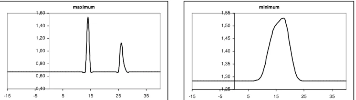
The model is based on the hypothesis that temperature is the main influential factor, in this way a pattern is defined by the daily maximum and minimum temperature values, all other factors (like trophic and other interpopulational interactions) appear concealed inside this factor. We have also presumed that the temperature reaction curve is the result of the sum of optimum curves because optimum temperature curves of the different species, of their different stages of development and perhaps their different subpopulations are summed up. In our model the value of the index changes from the first sampling day (giving the first value) according to a multiplier depending on daily maximum and minimum temperature (oC) values, by following this formula:
CIIt=RT.CIIt-1 (Eq. 1)
where CIIt is the value of the index at time „t” and RT is the growth rate depending on temperature. The temperature reaction curve is the result of the sum of two normal distribution curves (Fig. 1). Standard deviation and mean value of the distributions as well as the value of an added constant are curve is the result of two normal distribution ierges of development, pherhaps their different subpopu parameters of the model.
Parameters are optimized with the help of the Solver of MS Excel.
maximum
0,40 0,60 0,80 1,00 1,20 1,40 1,60
-15 -5 5 15 25 35
minimum
1,25 1,30 1,35 1,40 1,45 1,50 1,55
-15 -5 5 15 25 35
Figure 1.The reaction curve of CII: the value of RT multiplier plotted against maximum and minimum temperature
Subsequently we ran the model-system with the daily data series of climate change scenarios. The model was launched from the 90th to 135th day of the year because the samples fall into this period in all three years. OMSZ supplied us with meteorological data observed at the station of Fonyód, the station closest to the sampling site.
We used three data series of daily temperature specified for the period of 2070-2100.
We employed the database of PRUDENCE EU project [4] namely A2 and B2 scenarios of „HadCM3” climate change model ran by Hadley Centre (HC) and the run results of the Max Planck Institute (MPI) for A2 scenario. The daily data series were downscaled for the region of Zalaegerszeg and Siófok, the nearest observation stations. Being the result of the run of the above mentioned three different scenarios, the daily data series include 31 run years in both three cases.
The supervention of the yearly maximum CII value was used as an indicator for the statistical analysis of the modelling results.
Results and discussion
Overview of macroinvertebrates, their seasonal patterns and diversity relations based on field observation
Considering body volume, Tubificidae were represented in the greatest amounts in benthic ooze and Limnomysis benedeni in the water body. Furthermore, the number of Chironomidae and Cladocera specimen were prominent. The average numbers of individuals of taxa are shown in Table 1.
In some cases identification at a species level is not as yet finished. Tubificidae species are mostly Pothamotrix spp. and Branchiura sowerbii Beddard. We identified the larval and juvenile stages of fishes (Cyprinidae) but identification at species level happened in a few cases only. In most cases species are presuably Rutilus rutilus L., Scardinius erythrophthalmus L. or Alburnus alburnus L (one specimen might be Rhodeus sericeus amarus Bloch).
Table 1.Average numbers of individuals of the observed taxa in the examined years (total number of individuals divided by the number of sampling dates in the given year)
Taxa 2002 2003 2004
HYDROZOA
Hydra circumcincta Shulze 0.0 0.5 0.7
OLIGOCHAETA
Tubificidae 91.1 208.2 177.4
Pristina sp. 6.1 15.7 67.3
HIRUDINEA
Piscicola geometra L. 1.3 0.8 4.3
Glossiphonia heteroclita L. 0.0 0.2 4.1
Erpobdella octoculata L. 0.0 0.2 0.6
Helobdella stagnalis L. 0.4 0.5 1.3
BIVALVIA
Dreissena polymorpha Pall. 2.7 1.5 3.9
Pisidium sp. 0.0 0.1 0.0
GASTROPODA
Acroloxus lacustris L. 0.6 7.1 12.4
(other) Gastropoda 0.1 0.1 0.7
ARACHNOIDEA
Hydrachnidae 0.0 0.8 0.7
Araneidea 0.3 0.4 0.4
Taxa 2002 2003 2004 CRUSTACEA
Limnomysis benedeni Czern. 112.3 34.8 186.9
Dikerogammarus sp. 4.2 2.2 3.9
Corophium curvispinum G.O.Sars 2.8 1.2 6.3
Argulus sp. 1.5 0.5 0.3
Leptodora kindtii Focke 43.3 1.7 0.4
(other) Cladocera 64.4 76.1 35.4
Asellus aquaticus L. 0.0 0.2 0.7
Copepoda 4.2 1.4 1.0
COLLEMBOLA 0.0 0.0 0.1
EPHEMEROPTERA
Caenidae 0.0 1.5 5.3
Baetidae 0.3 11.9 24.3
ODONATA
Ischnura sp. 0.1 5.2 6.1
Anisoptera 0.0 0.0 0.1
HETEROPTERA
Aquarius paludum paludum Fab. 0.1 0.5 0.0
(other) Gerridae 0.1 0.5 0.1
Micronecta meridionalis Costa. 0.0 0.2 0.0
Sigara sp 0.0 1.6 0.0
Sigara striata L. 0.0 0.3 0.4
(other) Corixidae 0.0 0.3 0.0
Microvelia sp 0.9 3.0 27.9
Microvelia reticulata Scholtz. 0.0 1.0 0.0
Mesovelia furcata Mulsant & Rey. 0.1 0.1 0.3
Ranatra linearis L. 0.0 0.0 0.1
HOMOPTERA (Aphidinea) 0.0 2.0 1.1
COLEOPTERA 0.4 0.5 0.6
TRICHOPTERA
Hydroptilidae 0.0 0.5 0.0
Polycentropodidae 0.1 0.0 0.0
Limnephilidae 0.1 0.8 1.1
(other) Trichoptera 0.0 0.0 0.1
DIPTERA
Chironomidae 42.8 35.8 33.9
Ceratopogonidae 0.8 2.5 0.6
Tipulidae 0.0 0.2 0.1
Tabanidae 0.0 0.0 0.3
Syrphidae 0.0 0.0 0.1
"Diptera puparium" 1.1 1.2 2.6
"Diptera imago" 0.6 0.8 0.9
PISCES (Cyprinidae) 0.8 2.2 5.0
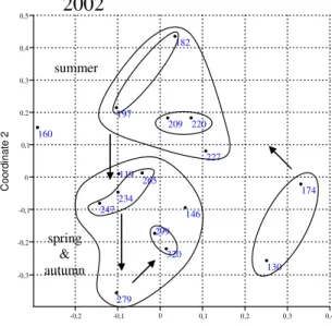
In order to explore temporal patterns we used several ordination and classification methods yielding very similar results. We present our results in ordination plots using NMDS with “Jaccard” similarity measure (Fig. 2).
In the ordination plots it is well observable, that the coenological states show a cyclic change throughout the growing season, thus expressing seasonality. Still, in 2002, no true trajectory could be detected. The most irregular groups fall into the period of the beginning of the season, when samples had to be taken in strong waves. In one case (138th day) only the sampling of benthic ooze was successful, this may be regarded as an error. No problem of this kind appeared in the following two years, regular trajectory and well isolated groups are typical of these years.
In 2003, groups characterising the different periods of the year can be separated more minutely than in 2004, which might be the result of more frequent sampling.
119
130 146
160
174 182
197 209 220
227
234 247
265
279 299
320
-0,2 -0,1 0 0,1 0,2 0,3 0,4
Coordinate 1
-0,3 -0,2 -0,1 0 0,1 0,2 0,3 0,4 0,5
summer
spring
&
autumn
Coordinate 2
2002
90
112 123
145 160 177
194 224 207
243 292 260
313
-0,3 -0,2 -0,1 0 0,1 0,2 0,3 0,4
Coordinate 1 -0,2
-0,1 0 0,1 0,2 0,3
Coordinate 2
spring
early summer late summer
autumn
2003
108
182 151
212
236
279 334
-0,2 -0,1 0 0,1 0,2 0,3 0,4
Coordinate 1
-0,4 -0,3 -0,2 -0,1 0 0,1 0,2 0,3 0,4 0,5 0,6
Coordinate 2
late autumn spring & early
summer
late summer & early autumn
2004
Figure 2. Change of the coenological state of the macroinvertebrate assembly and similarity pattern of dates (ordination, NMDS, Jaccard index), in the three years examined (2002, 2003,
2004). Serial numbers of sampling dates are shown.
The frequent and abundant morphons (all Tubificidae and Chironomidae, most body size categories of Limnomysis benedeni and Dikerogammarus sp. of medium size) were found throughout the year. Early spring proved to be the poorest in morphons in all three years, larger specimen of the frequent species characterise this period (larvae of Chironomidae and Limnomysis benedeni). In 2002, the early spring group is not so isolated which might be the result of the relatively late date of the first sampling (29th April) and the interfering effect of extreme weather conditions. Larval and juvenile fish are typical in the early summer. The largest numbers of morphons were observed late in
the summer (e.g. most Heteroptera, larvae of Ephemeroptera, Odonata and Trichoptera).
In the autumn again, less morphons could be detected (mainly zebra mussel and snails in most body sizes, imago of Sigara striata) and late in the autumn, we only found larger specimens of even less macroinvertebrate taxa (e.g. Piscicola geometra).
To compare diversity relations between three years, we applied Rényi’s diversity ordering based on morphons (Fig. 3). 2002 proved to be the least diverse year but it is not possible to order because its diversity profile intersects with the one of 2003. Based on the position and shape of the profiles we may assume that 2003 was definitely richer in rare morphons but 2002 in dominant morphons. The year 2004 was the most diverse in every domain of the scale parameter, but 2003 is very close if we consider rare morphons.
Figure 3.Diversity profiles of the examined three years (Rényi’s diversity ordering) For the demonstration of annual diversity trends we plotted the Shannon Diversity Index and Berger–Parker Dominance Index (Fig. 4). The years 2002 and 2003 are very similar in many respects: considerable decline can be observed in June (while the dominance index is increasing) and the most diverse date is in August. However, in 2002, the diversity value remains high until the end of autumn while in 2003, there is a drastic decline during this period (as the dominance index increases). Extremely high dominance values were recorded during this droughty year compared to the other years.
The most diverse period in 2003 coincides with the appearance of Najas marina stands, reaching a higher maximum diversity value than in 2002 when reed-grass stands were not present. These observations call attention to the importance of reed-grass.
Phenomena observed in 2004 confirm this theory, as high diversity values were recorded from the beginning of summer until the end of autumn, with the highest diversity value in October. Potamogeton perfoliatus stands were present during the whole growing season and in October a significant amount of reed-grass accumulated in front of the emergent macrophyte stands. The rule of dominant macroinvertebrates characterizes the beginning and the end of the growing season.
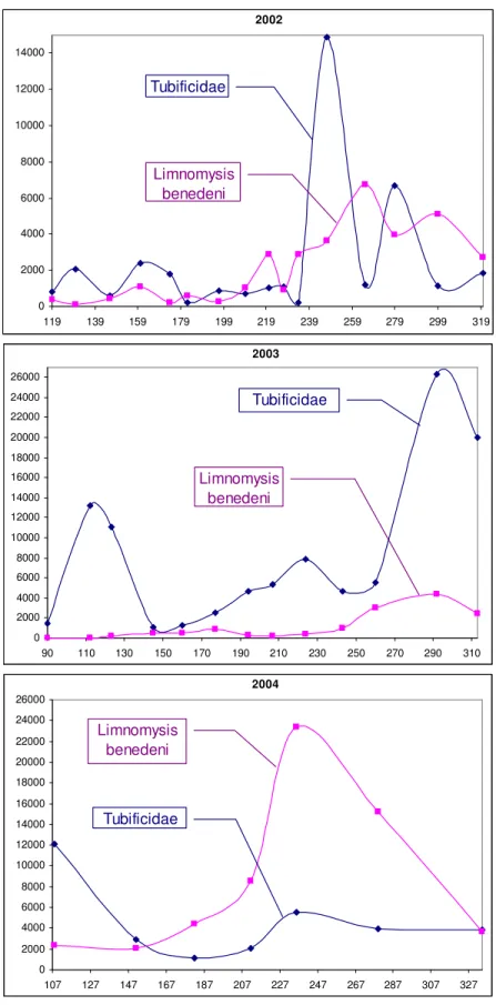
The seasonal dynamics of the two most abundant macroinvertebrate taxa are shown in (Fig. 5). The year 2002 was quite diversified: Tubificidae were more dominant until the end of June, then the quantity of the two macroinvertebrate taxa were roughly equal, that was followed by a period in which the alternate peaks of the two macroinvertebrate taxa appeared.
2002
0,00 0,50 1,00 1,50 2,00 2,50
1 2 3 4 5 6 7 8 9 10 11 12 13 14 15 16
0,00 0,10 0,20 0,30 0,40 0,50 0,60 0,70
Shannon
Berger-Parker
2003
0,00 0,50 1,00 1,50 2,00 2,50 3,00 3,50
1 2 3 4 5 6 7 8 9 10 11 12 13
0,00 0,10 0,20 0,30 0,40 0,50 0,60 0,70 0,80 0,90
Shannon
Berger-Parker
2004
0,00 0,50 1,00 1,50 2,00 2,50 3,00
1 2 3 4 5 6 7
0,00 0,05 0,10 0,15 0,20 0,25 0,30 0,35 0,40 0,45 0,50
Shannon
Berger-Parker
Figure 4.Temporal change of the Shannon Diversity Index and Berger-Parker Dominance Index in the years 2002, 2003 and 2004
2002
0 2000 4000 6000 8000 10000 12000 14000
119 139 159 179 199 219 239 259 279 299 319
Tubificidae
Limnomysis benedeni
2003
0 2000 4000 6000 8000 10000 12000 14000 16000 18000 20000 22000 24000 26000
90 110 130 150 170 190 210 230 250 270 290 310
Tubificidae
Limnomysis benedeni
2004
0 2000 4000 6000 8000 10000 12000 14000 16000 18000 20000 22000 24000 26000
107 127 147 167 187 207 227 247 267 287 307 327
Tubificidae Limnomysis
benedeni
Figure 5. Seasonal changes in the biovolume values (mm3) of Limnomysis benedeni and Tubificidae over three years (the serial numbers of days are shown on axis x)
The quantity of Tubificide was larger in the extremely droughty year of 2003, while in 2004, the volume of Limnomysis benedeni was significantly higher from the beginning of the summer.
Based on these characteristic facts it can be presumed, that the extremely low water level is favourable primarily for benthic organisms, mainly the detritivorous Tubificidae, while a higher level is to the advantage of the zoophagous Limnomysis benedeni preferring waters with more plants. All this is confirmed by the fact that the highest biovolume value of Tubificidae was recorded on 19th October 2003 when the water level of Lake Balaton was the lowest.
A weather-dependent simulation model of the seasonal changes of Coenological Intensity Index (CII) and the comparison of climate change scenarios
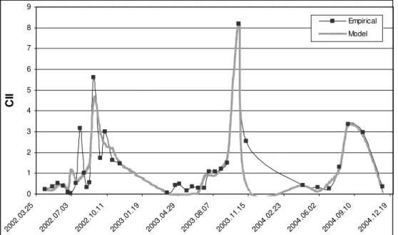
The temporal changes of the observed and the simulated values of CII over three years are shown in (Fig. 6). In the figure it can be clearly seen, that the model values fit well to the observed ones. As the temperature reaction curve of the model is practically the result of the sum of two normal distributions, two theoretical populations are enough to describe the temporal trends of CII characterising the whole assembly under examination. This might be in connection with our earlier conclusion, that there were two determinant groups in the examined macroinvertebrate population: Tubificidae and Limnomysis benedeni [20].
0 1 2 3 4 5 6 7 8 9
2002.03.25 2002.07.03
2002.10.11 2003.01.19
2003.04.29 2003.08.07
2003.11.15 2004.02.23
2004.06.02 2004.09.10
2004.12.19
CII
Empirical Model
Figure 6.The observed and the simulated values of CII during the three examined years
We ran the model for the three available daily data series of A2 and B2 scenarios, examining 31 running year each case. We considered the date of the supervening of the maximum value of CII (on which day of the year it occurs) as an indicator and the results of a one-way ANOVA for this indicator showed a significant difference between the scenarios (Table 2). The results of Tukey’s pairwise comparison (Table 3) proved
the A2 scenario of the Max Planck Institute to be significantly different from the A2 and B2 scenarios of the Hadley Centre, the latter two are showing a considerable similarity.
Table 2.The ANOVA table of the Variance Analysis made for the date of the supervening of the maximum values during the model ran for the three scenarios.
SS df MS F p (same)
Between Gr. 1.26E+05 2 6.31E+04 16.24 9.49E-07 Within Gr. 3.50E+05 90 3.88E+03
Total 4.76E+05 92
Table 3.The results of Tukey’s pairwise comparison (Tukey-test value / p(same)) A2 (HC) B2 (HC) A2 (MPI)
A2 (HC) 0.9817 0.000119
B2 (HC) 0.2594 0.000112
A2 (MPI) 6.847 7.106
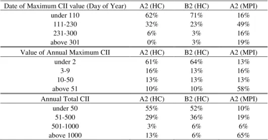
CII reached it’s maximum in the second half of the years under survey, between the end of August and the beginning of October (in 2002 on the 247th day in the beginning of September, in 2003 on the 292nd day in the beginning of October and in 2004 on the 236th day in the end of August). If we examine the supervening of the maximum values based on different scenarios (Table 4) we find these days shifting to earlier dates as much as to the beginning of the year. This phenomenon is particularly prominent in the case of the Hadley Centre scenarios, where in most of the 31 predicted years the date of maximum value falls to early spring. The A2 scenario of the Max Planck Institute also indicates a shift of this day to earlier dates, but in most cases this means dates in early summer rather than early spring.
Table 4.Table of the attributes of the model fitted to the 31 projected years of the A2 and B2 scenarios of Hadley Centre (HC) and the Max Planck Institute (MPI). The first column indicates the intervals of the year (expressed in serial numbers of the day of the year) and intervals of CII. In the other cells the percentage of the projected 31 years falling to the given interval is shown, considering the date of the supervening of the annual maximum CII value, the value of annual maximum and the annual total CII.
Date of Maximum CII value (Day of Year) A2 (HC) B2 (HC) A2 (MPI)
under 110 62% 71% 16%
111-230 32% 23% 49%
231-300 6% 3% 16%
above 301 0% 3% 19%
Value of Annual Maximum CII A2 (HC) B2 (HC) A2 (MPI)
under 2 61% 64% 13%
3-9 16% 13% 16%
10-50 13% 13% 13%
above 51 10% 10% 58%
Annual Total CII A2 (HC) B2 (HC) A2 (MPI)
under 50 55% 52% 10%
51-500 29% 36% 19%
501-1000 3% 6% 6%
above 1000 13% 6% 65%
With the help of Table 4. we can understand the differences between the scenarios based on an annual maximum CII and annual total CII values. It is obvious that the scenario of the Max Planck Institute definitely differs from the two scenarios of Hadley Centre regarding both indexes. The former predicts much higher maximum values then the ones observed (CII being between 3 and 10) but the latter ones forecast a shift towards regions lower then the observed values in most cases. The annual total quantity shows similar trends: the scenario of the Max Planck Institute predicts much higher values than the others.
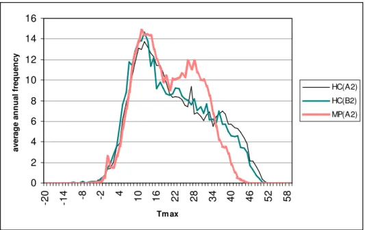
These features may clearly be explained by the difference between the temperature data series of the scenarios. The data series of the A2 scenario of the Max Planck Institute significantly differs from those of the two scenarios of Hadley Centre regarding either maximum (Fig. 7) or minimum temperature values (Fig. 8.) while no significant difference between the A2 and B2 scenarios of the latter institute can be observed.
This means the data of the runs of the Hadley Centre contain a higher number of extremely high temperatures but also forecast lower minimum values. The data of the Max Planck Institute are comparatively less deviated.
Confronting all this with the results of our CII model we can presume that a shift towards extreme weather leads to a fall of the index values regarding either maximum or annual total quantities. Less extreme scenarios with lower summer maximum temperature values may cause an increase of index value.
0 2 4 6 8 10 12 14 16
-20 -14 -8 -2 4 10 16 22 28 34 40 46 52 58
Tm ax
average annual frequency
HC(A2) HC(B2) MP(A2)
Figure 7. Annual mean frequency of the maximum temperature values of A2 scenario of the Max Planck Institute (MPI) and for A2 and B2 scenarios of Hadley Centre (HC), downscaled
for the region of the Siófok Meteorological Station
0 2 4 6 8 10 12 14 16 18 20
-20 -14 -8 -2 4 10 16 22 28 34 40 46 52 58
Tm in
average annual frequency
HC(A2) HC(B2) MP(A2)
Figure 8.Annual mean frequency of the minimum temperature values of A2 scenario of Max Planck Institute (MPI) and for A2 and B2 scenarios of Hadley Centre (HC), downscaled for the
region the Siófok Meteorological Station
Summary and conclusion
We attempted to explore seasonal patterns in a higher scale with the help of our series of samplings executed over several years at a site located in Lake Balaton, characterised by a vegetation of reed and reed-grass. The results call attention to the importance of more frequent sampling in order to explore groups characteristic for certain periods of the year in detail. In view of the final exclusion of deviations presumably caused by extreme weather events in 2002 the similarity (standardity) of the prevailing weather conditions for the time of sampling should gain greater attention. In light of all this, continued sampling shall lead us to a more detailed description of a circle of changes of states expressing seasonality, making possible a separation of morphon groups – or, using the classic term of coenology [1], aspects – characterising the different periods of the year [7].
Changes of water level and the presence of reed-grass vegetation had great influence on macroinvertebrate fauna. The effect of reed-grass was most prominent in increasing diversity, and that of decreasing water level in the stronger dominance of Tubificidae.
To model seasonal dynamics of macroinvertebrates we defined a „Coenological Intensity Index”, a combined index expressing the number of individuals, body volume and diversity. We created a model based exclusively on daily temperature values, capable of producing data series fitting well to the empirical values of CII. We ran the model for the data series predicted by the available A2 and B2 scenarios for the period between 2070-2100. Our results show that CII will reach its maximum much earlier, quite in the beginning of the year instead of the early autumn dates observed in recent years. However, the scenarios give different answers to the question of whether the total CII values will increase or decrease. These differences may clearly be explained by the
difference between the temperature data series of the institutes. We can admit, that in the case of scenarios forecasting higher maximum and lower minimum values the value of the index will decrease.
In our modelling work we use series of detailed data collected over a period of three years. The utilization of longer data series would make trophic approach possible e.g.
through the modelling of trophical guilds. With the modelling of combined groups, dominant species and using the method introduced in our study we might get a much more complex picture of the possible outcomes of climate change.
Acknowledgements. This research was supported by the projects OTKA T042583 and NKFP 6-00079/2005.
REFERENCES
[1] Balogh, J. (1953): A zoocönológia alapjai. [Grundzünge der zoozönologie] – Akadémiai Kiadó, Budapest.
[2] Bíró, K., Gulyás, P. (1974): Zoological investigations in the open water Potamogeton perfoliatus stands of Lake Balaton. – Annal. Biol. Tihany 41: 181-203.
[3] Entz, B. (1947): Qualitative and quantitative studies in the coatings of Potamogeton perfoliatus and Myriophillum spicatum in Lake Balaton. – Magyar Biológiai Kutató Intézet Munkái 17: 17-37.
[4] Christensen, J.H. (2005): Prediction of Regional scenarios and Uncertainties for Defining European Climate change risks and Effects. Final Report. DMI, Copenhagen.
[5] Fodor, N., Kovács, G.J. (2003): Sensitivity of 4M maize model to the inaccuracy of weather and soil input data. – Applied Ecology and Environmental Research 1(1-2): 75- 85.
[6] Gaál, M., Schmidtke, J., Rasch, D., Schmidt, K., Neemannn, G., Karwasz, M. (2004):
Simulation experiments to evaluate the robustness of the construction of monitoring networks. – Applied Ecology and Environmental Research 2(2): 59-71.
[7] Hufnagel, L., Gaál, M. (2005): Seasonal dynamic pattern analysis service of climate change research. – Applied Ecology and Environmental Research 3(1): 79-132.
[8] Jordán, F. (2003): Comparability: the key to the applicability of food web research. – Applied Ecology and Environmental Research 1(1-2): 1-18.
[9] Kovács, M. (1991): A Balaton növényzetének vizsgálata 1900-tól napjainkig. – In: Bíró, P. (ed.) 100 éves a Balaton-Kutatás. Tihany. 63-68.
[10] Ladányi, M., Horváth, L., Gaál, M., Hufnagel, L. (2003): An agro-ecological simulation model system. – Applied Ecology and Environmental Research 1(1-2): 47-74.
[11] Máté–Gáspár, G., Kovács, G.J. (2003): Use of simulation technique to distinguish between the effect of soil and weather on crop development and growth. – Applied Ecology and Environmental Research 1(1-2): 87-92.
[12] Muskó, I. B., Balogh, Cs., Bakó, B., Leitold, H., Tóth, Á. (2004): Gerinctelen állatok szezonális dinamikája balatoni hínárosban, különös tekintettel néhány pontokáspi inváziós fajra. – Hidrológiai Közlöny, 84: 12-13.
[13] Ponyi, J. (1956): A balatoni hínárosok Crustaceáinak vizsgálata. – Állattani Közlemények 45: 107-121
[14] Rédei, D., Gaál, M., Hufnagel, L. (2003): Spatial and temporal patterns of true bug assemblages extracted with Berlese funnels (Data to the knowledge on the ground–living Heteroptera of Hungary, № 2). – Applied Ecology and Environmental Research 1(1-2):
115-142.
[15] Rédei, D., Harmat, B., Hufnagel, L. (2003): Ecology of the Acalypta species occurring in Hungary (Insecta: Heteroptera: Tingidae). – Applied Ecology and Environmental Research 2(2): 73-90.
[16] Rédei, D., Hufnagel, L. (2003): The species composition of true bug assemblages extracted with Berlese funnels (Data to the knowledge on the ground–living Heteroptera of Hungary, № 1). – Applied Ecology and Environmental Research 1(1-2): 93-113.
[17] Ryan, P.D., Harper, D.A.T., Whalley, J.S. (1995): PALSTAT, Statistics for paleontologists. – Chapman & Hall (now Kluwer Academic Publishers).
[18] Singh, N.B., Khare, A.K., Bhargava, D.S., Bhattacharya, S. (2004): Optimum moisture requirement during Vermicomposting using Perionyx excavatus. – Applied Ecology and Environmental Research 2(1): 53-62.
[19] Sipkay, Cs. (2005): Módszertani esettanulmány mikrohabitatok zoocönológiai mintázatfeltárásához egy vízi makrogerinctelen közösségben. – VII. Magyar Biometriai és Biomatematikai Konferencia, Abstract Kötet: 46-47.
[20] Sipkay, Cs., Hufnagel, L. (2006): Makrogerinctelenek vizsgálata három jellegzetes balatoni mikrohabitatban. – Hidrológiai Közlony 86(6): 106-109.
[21] Sipkay Cs., Hufnagel L. (2006): Szezonális dinamikai folyamatok egy balatoni makrogerinctelen együttesben. Acta Biologica Debrecina Supplementum Oecologica Hungarica 14: 211-222.
[22] Sipkay, Cs., Hufnagel, L., Gaál, M. (2005): Zoocoenological state of microhabitats and its seasonal dynamics in an aquatic macroinvertebrate assembly (Hydrobiological case studies on Lake Balaton, №.1) – Applied Ecology and Environmental Research 3(2): 107- 137.
[23] Sipkay, Cs., Nosek, J., Oertel, N., Vadadi-Fülöp, Cs., Hufnagel, L. (2007):
Klímaváltozási szcenáriók elemzése egy dunai copepoda faj szezonális dinamikájának modellezése alapján. – “Klíma21” 49: 80-90.
[24] Vadadi-Fülöp Cs., Hufnagel L. (2007): Klímaváltozási szcenáriók értékelése egy kerti tó zooplankton közösségének szezonális dinamikájának alapján. Hidrológiai Közlöny (in press)
[25] Vadadi-Fülöp, Cs., Sipkay, Cs., Hufnagel, L. (2007): Klímaváltozási szcenáriók értékelése egy szitakötőfaj (Ischnura pumilio, Charpentier, 1825) szezonális dinamikája alapján – Acta Biologica Debrecina, Oecol. Hung. 16: 211-219.