Periodic orbits and global stability for a discontinuous SIR model with delayed control

(1)

(will be inserted by the editor)

Periodic orbits and global stability for a discontinuous SIR model with delayed control

Khalil Muqbel · Gabriella Vas · Gergely R¨ost

6 February 2020 Received: date / Accepted: date

Abstract We propose and analyse a mathematical model for infectious disease dynamics with a discontinuous control function, where the control is activated with some time lag after the density of the infected population reaches a threshold. The model is mathematically formulated as a delayed relay system, and the dynamics is determined by the switching between two vector fields (the so-called free and control systems) with a time delay with respect to a switching manifold. First we establish the usual threshold dynamics: when the basic reproduction number R0≤1, then the disease will be eradicated, while for R0>1 the disease persists in the population. Then, for R0>1, we divide the parameter domain into three regions, and prove results about the global dynamics of the switching system for each case: we find conditions for the global convergence to the endemic equilibrium of the free system, for the global convergence to the endemic equilibrium of the control system, and for the existence of periodic solutions that oscillate between the two sides of the switching manifold. The proof of the latter result is based on the construction of a suitable return map on a subset of the infinite dimensional phase space. Our results provide insight into disease management, by exploring the effect of the interplay of the control efficacy, the triggering threshold and the delay in implementation.

Keywords epidemiological model, non-smooth dynamical system, disease control, time delay, stability, periodic solution

Khalil Muqbel, Gergely Röst, Bolyai Institute, University of Szeged, Aradi vértanúk tere 1.,

Szeged H-6720, Hungary E-mail: rost@math.u-szeged.hu

Gabriella Vas

MTA-SZTE Analysis and Stochastics Research Group, Bolyai Institute, University of Szeged

Aradi v´ertan´uk tere 1., Szeged H-6720, Hungary

(2)

1 Introduction

Switching models have been used recently in the compartmental models of mathematical epidemiology to analyze the impact of control measures on the disease dynamics. For example, it has been observed that if the treatment rate [12] or the incidence function [1] is non-smooth, that may lead to various bifurcations. These sharp changes occur in [1] and [12] when the total population, or the infected population reaches a threshold level. Such a sudden change may even be discontinuous, for example due to the implementation or termination of an intervention policy such as vaccination or school closures.

Mathematically, such situations are described by Filippov systems, when the phase space is divided into two (or more) parts and the system is given by different vector fields in each of those parts. Examples include sudden changes in vaccination [9,13], hospitalization [16], transmission [14], travel patterns [7], or the combination of several effects [15]. They have been used for vector borne diseases as well [17].

An overview of the basic theory and applications of switching epidemiological models can be found in [8]. Many of the mathematical challenges appear due to the incompatible behaviours of the vector fields at their interfaces, on the so-called switching manifold.

Switching systems typically assume that the change in the vector field occurs immediately whenever the switching manifold is touched, for example, a threshold in a population variable is reached. However, in reality, implementing a policy may have some time lag, hence it is natural to consider the situation when we switch to the new vector field with some delay after the trajectory intersected the switching manifold. These systems are called delayed relay systems [10], and they are of different mathematical nature than the Filippov systems.

Delayed relay systems have been applied to an SIS model [6], where explicit periodic solutions were constructed for the case of a delayed reduction in the contact rate after the density of infection in the population passed through a threshold value. The dynamics of this discontinuous system was different from its continuous counterpart [5],[4], showing that it is worthwhile to analyse the dynamics of epidemiological systems with delayed switching. The simplistic SIS model of [6] could be reduced to a scalar equation, and here we initiate the study of more realistic and more complex compartmental models in this context.

In particular, in this paper our starting point is an SIR model with switching, which has been thoroughly investigated in [14] by Xiao, Xu, and Tang. The model represents circumstances when intervention measures are taken only when the density of infectious individuals is exceeding a certain threshold value. This is expressed by a discontinuous incidence rate, more precisely, the intervention causes a drop in the transmission rate. They showed that the solutions ultimately approach one of the two endemic states of the two structures (the free and the control system), or the so-called sliding equilibrium located on the switching surface, depending on the threshold level.

Here we introduce the possibility of a time delay in the threshold policy. We prove several global stability theorems for the system with delay. An important difference in the dynamics is that while in the model of [14] the existence of limit cycles was excluded, for our model periodic orbits exist, and we prove that by constructing a Poincar´e-type return map on a special subset of the phase space.

These periodic solutions oscillate around the threshold level. On the other hand,

(3)

the sliding mode control in [14] does not appear in our system. Our results con- tribute to the development of a systematic way of designing simply implementable controls that drive the dynamics towards disease control or mitigation.

2 Model description

The population N is divided into three compartments: susceptible (S), infected (I) and recovered (R). All individuals are born susceptible, and the birth rate is µ >0 for each compartment. The death rate is alsoµfor each class, and hence the total populationN=S+I+R is constant, which we normalize to unity,N = 1.

Although in classical SIR models with mass action incidence, the new infections occur with some constant transmission coefficient β > 0, here we assume that the transmission coefficient depends on the number of infected individuals: If the density of infected individuals reaches a threshold levelk∈(0,1), then the society implements certain control measures, and thereby the transmission rate is reduced fromβ to (1−u∗)β with u∗∈ (0,1). The constant u∗ represents the efforts and the efficacy of the control measures. It is reasonable to assume that this reduction takes place with a time delay τ > 0. If the density of the infected individuals becomes less than k, then the control measures are stopped, again with delay τ >0. Infected individuals recover with rateγ >0, and full lifelong immunity is assumed upon recovery. With these assumptions above, we obtain the following SIR model with delay:

dS(t)

dt = µ−µS(t)−[1−u(I(t−τ))]βS(t)I(t), dI(t)

dt = [1−u(I(t−τ))]βS(t)I(t)−γI(t)−µI(t), dR(t)

dt = γI(t)−µR(t),

(1)

where

u(I) = (

0 ifI < k,

u∗ ifI≥k, (2)

k∈(0,1) andu∗∈(0,1).

In the special caseτ = 0 we obtain a model studied in [14].

A dynamical system is called a delayed relay system [10], if it is governed by a differential equation of the form

dx(t) dt =

(

f¹(x(t)) ifg(x(t−τ))<0, f²(x(t)) ifg(x(t−τ))≥0,

where τ > 0, and f¹, f² are Lipschitz continuous. The switching function g is typically a piecewise smooth Lipschitz continuous function. The set{x:g(x) = 0} is called the switching manifold.

Let (Sysd) denote the system consisting of the first two equations of (1). We consider only these two equations as they are independent of the third one in (1).

(4)

Note that (Sysd) is a delayed relay system withx= (S, I), f¹(S, I) =

f₁¹(S, I) f₂¹(S, I)

T

=

µ−µS−βSI βSI−γI−µI

T

,

f²(S, I) =

f₁²(S, I) f₂²(S, I)

T

=

µ−µS−(1−u∗)βSI (1−u∗)βSI−γI−µI

T (3) andg(S, I) =I−k. Now the switching manifold is the set{(S, I) :I=k}.

Hereinafter (Sysf) denotes the free system

(S⁰(t), I⁰(t)) =f¹(S(t), I(t)), and (Sysc) is for the control system

(S⁰(t), I⁰(t)) =f²(S(t), I(t)).

Let us emphasize that these are 2-dimensional systems consisting of theS- andI- equations of a classical ordinary SIR model. The transmission rate isβfor (Sys_f), and it is (1−u∗)βfor (Sysc).

As it is well-known, the set

∆={(S, I)∈[0,1]²: S+I≤1} (4) is positively invariant for both (Sysf) and (Sysc). For all (S0, I0)∈∆and for both

∗ ∈ {f, c}, let

(S∗, I∗) = (S∗(·;S0, I0), I∗(·;S0, I0)) denote the solution of (Sys∗) with

S∗(0) =S∗(0;S0, I0) =S0 and I∗(0) =I∗(0;S0, I0) =I0.

Solution (S∗, I∗) exists on the positive real line. It is also important that ifI0= 0, then I∗(t) = 0 for allt≥0. ConditionI0>0 guarantees that I∗ remains positive on the positive real line. In other words,

∆1={(S, I)∈∆:I >0} (5)

is positively invariant w.r.t. both (Sys_f) and (Sysc).

Because of the delayτ, the phase space for (Sys_d) has to be chosen as X ={(S0, ϕ)∈[0,1]×C([−τ,0],[0,1]) :S0+ϕ(0)≤1}.

Given any (S0, ϕ)∈X, the solution (S, I) = (S(·;S0, ϕ), I(·;S0, ϕ)) of (Sys_d) is a pair of real functions with the following properties:Sis defined and continuous on [0,∞) with S(0) =S0, I is defined and continuous on [−τ,∞) withI|_[_−τ,_0]=ϕ, furthermore, (S, I) satisfies the integral equation system

S(t) =S0+ Z t

0

{µ−µS(ξ)−[1−u(I(ξ−τ))]βS(ξ)I(ξ)}dξ, I(t) =ϕ(0) +

Z t

0

{[1−u(I(ξ−τ))]βS(ξ)I(ξ)−γI(ξ)−µI(ξ)}dξ for allt >0.

(5)

It is obvious that the solutions of (Sysd) are absolutely continuous, and the first two equations in (1) are satisfied almost everywhere. Throughout the paper S⁰(t) andI⁰(t) will mean the right-hand derivative whenI(t−τ) =k; this will not cause any confusion.

For all t≥0, let It denote the element of C([−τ,0],[0,1]) defined by It(ξ) = I(t+ξ),ξ∈[−τ,0].

Consider the following subset ofX:

X₀={(S₀, ϕ)∈X: [−τ,0]3t7→ϕ(t)−k∈Rhas a finite number of sign changes}.

In this paper we only study solutions with initial data inX0. A further subset of X is

X₁={(S₀, ϕ)∈X₀:ϕ(0)>0},

the collection of endemic states, when the disease is present in the population. We will show in Section 4 that bothX₀ andX₁ are positively invariant for (Sys_d).

3 Equilibria

In case of the free system (Sys_f), the basic reproduction number is R0= ^β

γ+µ.

The reproduction number of the control system (Sysc), what we call control reproduction number, is given by

Ru∗= (1−u∗)β

γ+µ = (1−u∗)R0.

Next we recall the equilibria and their stability properties for the ordinary systems (Sys_f) and (Sysc).

The disease-free equilibrium for both (Sys_f) and (Sysc) is E^∗0= (S0^∗, I0^∗)∈∆, where S0^∗= 1 andI0^∗= 0. The endemic equilibrium for (Sysf) is

E^∗₁= (S₁^∗, I₁^∗)∈∆, where S₁^∗= 1 R0

andI₁^∗= ^µ

β(R0−1). It exists only ifR0>1.

It is known (see [3]) that E₀^∗ is globally asymptotically stable w.r.t the free system (Sysf) ifR0 ≤1, and it is unstable if R0 >1. The endemic stateE₁^∗ is asymptotically stable w.r.t (Sys_f) ifR0>1,and its region of attraction is∆1.

The endemic equilibrium for (Sysc) is E^∗₂= (S₂^∗, I₂^∗)∈∆, where S₂^∗= 1

Ru∗

andI₂^∗= ^µ

(1−u∗)β(Ru∗−1). It exists forRu∗>1.

(6)

E^∗₂is asymptotically stable w.r.t (Sysc) and attracts∆1ifRu_∗>1.The disease free equilibriumE₀^∗ is globally asymptotically stable w.r.t (Sysc) if Ru∗ ≤1, and it is unstable ifRu∗>1.

Next we examine what are the equilibria for (Sys_d).

For all I^∗ ∈ [0,1], let I^∗ also denote the constant function in C([−τ,0],[0,1]) with value I^∗. This will not cause any confusion but ease the notation. If we write (S^∗, I^∗)∈ ∆, then I^∗ is considered to be a real number in [0,1]. Notation (S^∗, I^∗)∈X0 means that I^∗ is an element ofC([−τ,0],[0,1]). In accordance, we may considerE^∗₀, E^∗₁ andE^∗₂ as elements ofX0.

(S^∗, I^∗)∈X₀ is an equilibrium for (Sys_d) if and only if (S^∗, I^∗)∈∆satisfies the algebraic equation system

0 =µ−µS^∗−[1−u(I^∗)]βS^∗I^∗,

0 = [1−u(I^∗)]βS^∗I^∗−γI^∗−µI^∗. (6) As above, we call an equilibrium (S^∗, I^∗) disease-free if I^∗ = 0, and endemic if I^∗>0.

By calculating the solutions of (6), we obtain the following result.

Proposition 1

The unique disease-free equilibrium for the delayed relay system (Sysd)is E₀^∗ ∈X0, and it exists for all choices of parameters.

If R0 ≤ 1, then there is no endemic equilibrium for (Sys_d). If R0 > 1, then we distinguish three cases.

(a) If

R0>1 and R0[µ−(µ+γ)k]< µ, (C.1) thenE₁^∗∈X₀ is the unique endemic equilibrium for(Sys_d).

(b) If

µ≤ R0[µ−(µ+γ)k]< µ/(1−u∗), (C.2) then there is no endemic equilibrium for(Sys_d).

(c) If

R0[µ−(µ+γ)k]≥µ/(1−u∗), (C.3) thenE₂^∗∈X₀ is the unique endemic equilibrium.

Note that if either (C.2) or (C.3) holds, then necessarily R0>1. In addition, conditions (C.1), (C.2) and (C.3) together cover the caseR0>1.

Proof It is easy to see that (S^∗,0) satisfies (6) if and only ifS^∗=S^∗₀= 1. Moreover, (S₀^∗, I₀^∗) = (1,0) is a solution of (6) without any restrictions on the parameters. So the first statement of the proposition is true.

We may now assume thatI∗>0 and thusS^∗<1. Let us divide (6) by (µ+γ) and examine the equivalent form

0 = ^µ

γ+µ(1−S^∗)−[1−u(I^∗)]R0S^∗I^∗, 0 = [[1−u(I^∗)]R0S^∗−1]I^∗.

(7)

AsI^∗6= 0, the second equation gives that

R0[1−u(I^∗)]S^∗= 1. (7) It comes from S^∗ < 1 and the definition of u that (7) cannot be satisfied if R0≤1, so in that case there is no endemic equilibrium.

If R0 > 1, then we need to distinguish two cases. If 0 < I^∗ < k and hence u(I∗) = 0, then one can easily see that (S^∗, I^∗) = (S₁^∗, I₁^∗).IfI^∗≥kandu(I∗) =u∗, then (S^∗, I^∗) = (S₂^∗, I₂^∗).

To complete the proof, we need to guarantee that 0< I₁^∗< kandI₂^∗≥k. Using β=R0(µ+γ),one can show that inequality

0< I1^∗= ^µ

β(R0−1)< k is satisfied if and only if

1<R0 and R0[µ−(µ+γ)k]< µ.

Similarly,I₂^∗≥k is equivalent to

R0[µ−(µ+γ)k]≥µ/(1−u∗).

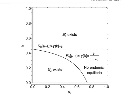
Statements (a)-(c) of the proposition follow from the calculations above. ut In Fig. 1 we divide the (k, u∗) plane into three regions acoording to Cases (a)- (c) of Proposition 1 in order to show the interplay between threshold levelk and control intensityu∗.

4 Construction of solutions

In this section we show that if (S0, ϕ)∈X0((S0, ϕ)∈X1), then the solution (S, I) exists, and (S(t), It)∈X₀ ((S(t), It)∈X₁) for eacht≥0.

First we need the following result for the ordinary systems (Sysf) and (Sysc).

Proposition 2 Let ∗ ∈ {f, c}. For any k ∈ (0,1) and any non-constant solution (S∗, I∗)of(Sys∗), the function

[0,∞)3t7→I∗(t)−k∈R has a finite number of zeros on each interval of finite length.

Proof We give a proof for the free system (Sys_f). The proof for (Sysc) is analogous.

Consider the second equation of (Sys_f):

I_f⁰(t) =βS_f(t)I_f(t)−(γ+µ)I_f(t) = (γ+µ) R0S_f(t)−1

I_f(t). (8) IfR0 ≤1 andI_f(t) =k ∈ (0,1) for somet≥0, then S_f(t)≤1−I_f(t)<1 and I_f⁰(t)<0. The statement is clearly true in this case.

Now assume that R₀>1. Recall from [3] that V(S, I) =S1^∗

S

S^∗₁ −log ^S S₁^∗

+I1^∗

I

I₁^∗ −log ^I I₁^∗

(8)

E₁^*exists

E₂^*exists No endemic equilibria R₀[μ-(μ+γ)k]=μ

R₀[μ-(μ+γ)k]= μ 1-u_*

0.0 0.2 0.4 0.6 0.8 1.0

u_*

k

Fig. 1: A 2-parameter bifurcation diagram giving the endemic equilibria in the (k, u∗) plane forR0>1. The parameters areγ= 0.25,β= 2.5 andµ= 0.4.

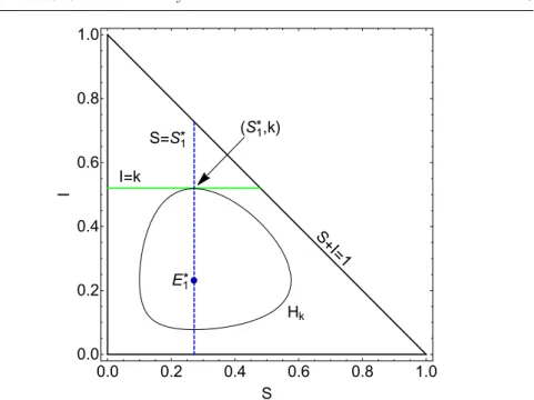
is a Lyapunov function for (Sys_f), and ˙V(S, I)<0 for all (S, I)∈∆1\ {E^∗₁}. For anyk∈(0,1)\ {I₁^∗}, consider the nontrivial level set

Hk=

(S, I)∈∆1: V(S, I) =S₁^∗+k−I₁^∗log ^k I₁^∗

,

which is a simple closed curve. The property ˙V(S, I)<0 guarantees thatint(H_k) is positively invariant for (Sysf), whereint(Hk) denotes the interior ofHk.

Observe that (S₁^∗, k)∈Hk. One can easily check that [0,1]3S 7→V(S, k)∈R has a strict minimum at S =S₁^∗, which implies that the segment I =k andH_k have no common point besides (S₁^∗, k). The segmentI=k is tangential toH_k at (S₁^∗, k), see Fig. 2.

We also see from (8) that ifI_f(t)>0 for somet∈R, then

I_f⁰(t) = 0 if and only if Sf(t) = 1/R0=S1^∗, (9) and

I_f⁰(t)>0 (I_f⁰(t)<0) if and only if Sf(t)> S₁^∗ (Sf(t)< S₁^∗). (10) A direct consequence of (9) is the following observation for a non-constant solution (Sf, If). If there exists ˜t ≥0 such that If ˜_t

= k andI_f⁰ ˜_t

= 0, then S_f ˜_t

=S₁^∗by (9). Due to the Lyapunov function, there are no periodic solutions, hence there is not6= ˜tsuch that (S_f(t), I_f(t)) = (S₁^∗, k). This yields, again by (9), that ifI_f(t) =k for somet∈[0,∞)\ {˜_t}, thenI_f⁰(t)6= 0.

Now suppose for contradiction that for some k ∈(0,1) and non-constant solution (Sf, If), the function [0,∞) 3 s 7→ If(s)−k ∈ R has an infinite number

(9)

E₁^* S=S₁^* I=k

S+I=1 (S₁^*,k)

Hk

0.0 0.2 0.4 0.6 0.8 1.0

S

I

Fig. 2: The segmentI=kand the level setH_k of the Lyapunov functionV.

of zeros in a finite closed interval J ⊂[0,∞). Let B = {t∈ J:I_f(t) = k}. The compactness ofJ ensures thatB has an accumulation pointta inJ. Necessarily If(ta) =k.

Let ε > 0 be arbitrary. Next we show that B has elements t1 < t2 < t3 in (ta−ε, ta+ε) such that

I_f⁰(t1)<0, I_f⁰(t2)>0, I_f⁰(t3)<0,

I_f(t)< kfort∈(t₁, t₂) and I_f(t)> kfort∈(t₂, t₃).

One can prove this claim as follows. Either (ta−ε, ta) or (ta, ta+ε) contains elements of B arbitrary close to ta. Suppose (ta−ε, ta) is such an interval. By decreasingε, we may assume that the point ˜t(if exists) is not in (ta−ε, ta), and hence

I_f⁰(t)6= 0 for allt∈B∩(ta−ε, ta). (11) Choose any t1 ∈ B∩(ta −ε, ta) with I_f⁰(t1) < 0. It is easy to see that such t1

exists, otherwise we cannot have several zeros in (ta−ε, ta). Then one can give δ1>0 witht1+δ1< ta such thatIf(t)< kfort∈(t1, t1+δ1). AsB∩(t1+δ1, ta) is bounded and nonempty (actually it has an infinite number of elements), the infimumt2= inf{B∩(t1+δ1, ta)}exists. It is clear thatt1< t2< ta, andI_f(t2) =k by the continuity ofI_f. Observation (11) guarantees thatI_f⁰(t2)6= 0. It comes from the definition oft2 thatI_f(t)< kfor t∈(t1, t2) andI_f⁰(t2)>0. As next step, one can give δ2 > 0 such that t2+δ < ta and I_f(t) > k for t ∈ (t2, t2+δ2). Set t₃ = inf{B∩(t₂+δ₂, ta)}. Then t₃ satisfies the properties given in the claim. In the second case, whenB has infinite elements in (ta, ta+ε), we can findt3 first, thent2 andt1 in an analogous way.

(10)

We claim thatI_f⁰(ta) = 0, and thereforeSf(ta) =S₁^∗(that is,ta= ˜t). Indeed, if I_f⁰(ta) is positive (negative), thenI_f⁰(t) is positive (negative) for allt∈Bin a small neighbourhood oftaby the continuous differentiability ofI_f. This contradicts our previous claim. SoS_f(ta) =S^∗₁.

As the solution is non-constant, (S_f(ta), I_f(ta)) = (S₁^∗, k)6= (S₁^∗, I₁^∗), and we conclude that k 6= I₁^∗. We consider the case k > I₁∗. (The case k < I₁∗ can be handled in similarly.)

Recall that (Sf(ta), If(ta)) = (S^∗₁, k) is the intersection point of the segment I=kandH_k. We have seen that there existt1andt2arbitrary close totasuch that I_f(t1) =I_f(t2) =k,I_f⁰(t1)<0< I_f⁰(t2) andI_f(t)< k fort∈(t1, t2). Remark (10) implies thatS_f(t₁)< S₁^∗< S_f(t₂). We may also achieve (using the boundedness of S_f⁰ andI_f⁰) that (Sf(t), If(t)) is arbitrary close to (S^∗₁, k) on (t1, t2). This gives the existence oft∗∈(t1, t2) with (Sf(t∗), If(t∗))∈int(Hk). The positive invariance of int(H_k) then gives (S_f(t), I_f(t))∈int(H_k) for allt≥t∗ contradictingI_f(t2) =k.

This means that our initial assumption was wrong, and the proposition is true

also in theR0>1 case. ut

Now we ready to prove the positive invariance ofX₀.

Proposition 3 If(S0, ϕ)∈X0, then a unique solution(S, I)exists, and(S(t), It)∈ X0 for eacht≥0.

Proof Set

0 =t0< t1< ... < t_N₋₁< t_N =τ

such that ϕ(ξ)< kon intervals of the form (−τ+t2n,−τ+t2n+1) and ϕ(ξ)> k on intervals of the form (−τ+t2n−1,−τ+t2n), wheren∈[0, N/2] is an integer.

(We omit the case when ϕ(ξ) > k on (−τ +t2n,−τ +t2n+1) and ϕ(ξ) < k on (−τ+t2n−1,−τ+t2n) because that can be handled analogously.)

Under the assumptions above, I(t−τ)< k andu(I(t−τ)) = 0 fort∈(0, t₁).

Hence the solution (S, I) of (Sysd) coincides with a solution of (Sysf) on [0, t1]:

S(t;S0, ϕ) =S_f(t;S0, ϕ(0)), I(t;S0, ϕ) =I_f(t;S0, ϕ(0))

for t∈[0, t1]. SinceI(t−τ)> k and thus u(I(t−τ)) =u∗ for t∈(t1, t2), we see that

S(t;S0, ϕ) =Sc(t−t1;S(t1), I(t1)), I(t;S0, ϕ) =Ic(t−t1;S(t1), I(t1)) fort∈[t1, t2]. Similarly, (S, I) is given by a specific solution of (Sysf) or (Sysc) on all intervals of the form [tm−1, tm], wherem∈ {1, ..., N}. Hence the solution exists on [0, τ].

As the functions t7→ I_f(t)−k andt 7→ Ic(t)−k have finite number of sign changes on intervals of finite length by Proposition 2, we deduce thatt7→I(t)−k also admits a finite number of sign changes on [0, τ].

Iterating this argument first for [τ,2τ], then for all intervals of the form [jτ,(j+ 1)τ],j≥2, we see that the solution exists on the positive real line. The uniqueness of (S, I) comes at once from the uniqueness of solutions for (Sys_f) and (Sysc).

In addition, it is clear that t7→ I(t)−k has a finite number of sign changes on intervals of finite length. The way we obtain the solutions of (Sys_d) and the positive invariance of∆for (Sysf) and (Sysc) also imply thatS(t)∈[0,1],I(t)∈[0,1] and S(t) +I(t)≤1 for allt≥0. Summing up, (S(t), It)∈X0 for allt≥0. ut

(11)

Since the solutions of (Sysd) with initial data in X0 are determined by the solutions of (Sys_f) and (Sysc) as in the previous proof, and as the set ∆1 = {(S, I)∈∆:I >0}is positively invariant for both (Sys_f) and (Sysc), we see that X₁ is positively invariant for (Sys_d) too.

5 Threshold dynamics: disease extinction and persistence

Theorem 1 IfR0≤1, thenE^∗₀ is globally asymptotically stable for the delayed relay system(Sys_d)(that is,E^∗₀ is asymptotically stable and attracts X₀). IfR0>1, then E₀^∗ is unstable w.r.t.(Sysd), and the disease uniformly persists in the population.

Proof First note that the solutions of (Sys_d) coincide with the solutions of the free system (Sys_f) in a small neighbourhood ofE^∗₀. ThereforeE₀^∗is a stable equilibrium for (Sysd) if and only if it is stable for (Sysf).

LetR0≤1. We only need to prove the global attractivity ofE₀^∗onX0. Suppose for contradiction thatI(t) does not converge to 0 ast→ ∞for some solution (S, I).

By the second equation of (Sys_d), dI(t)

dt = (µ+γ){[1−u(I(t−τ))]R0S(t)−1}I(t)≤0,

that is,I is nonincreasing. AsI is nonnegative and does not converge to 0, necessarily there exists a constantc >0 such thatI(t)≥cfor allt≥0 andI(t)→cas t→ ∞. ThenS(t)≤1−cand

{[1−u(I(t−τ))]R0S(t)−1}I(t)≤ −c² for allt≥0. It follows that

I(T) =I(0) + (µ+γ) Z T

0

{[1−u(I(ξ−τ))]R0S(ξ)−1}I(ξ)dξ≤I(0)−(µ+γ)c²T, which impliesI(T)<0 for all sufficiently largeT, a contradiction. SoI(t)→0 as t→ ∞.

Next we prove that ifR0≤1, thenS(t)→1 ast→ ∞for all solutions (S, I). It is clear from the previous paragraph that there existsT(ε) for each ε >0 such thatI(t)< εfor allt≥T(ε).Then fort≥T(ε),

dS(t)

dt =µ−µS(t)−[1−u(I(t−τ))]βS(t)I(t)≥µ−µS(t)−εβS(t), which implies

lim inf

t→∞ S(t)≥ µ µ+εβ. Note thatε >0 can be arbitrary small. Thereby

lim inf

t→∞ S(t)≥µ µ = 1.

We know on the other hand thatS(t)≤1 for allt≥0.Summing up, limt→∞S(t) exists and equals one.

We have verified thatS(t)→1 andI(t)→0 ast→ ∞for every solution (S, I) ifR0≤1.

(12)

To show the persistence, let R0>1, and consider a solution withI(0)>0. If there exists arbitrarily largetwithI(t)≥k, then lim sup_t→∞I(t)≥k. Otherwise, there is a t∗ such that I(t)< k for all t > t∗. In this case, the solution follows (Sys_f) fort≥t∗+τ:

S(t) =Sf(t−t∗−τ;S(t∗+τ), I(t∗+τ)),

I(t) =I_f(t−t∗−τ;S(t∗+τ), I(t∗+τ)), t∈[t∗+τ,∞).

Then limt→∞I(t) = I₁^∗. In any case, we can conclude that lim sup_t→∞I(t) ≥ min{k, I₁^∗},which means uniform weak persistence. Since the solutions of (Sys_f) and (Sysc) both have uniformly bounded derivatives on∆, by the Arzel`a-Ascoli theorem our solution operatorsΦ(t) :X₀3(S₀, ϕ)7→(St, It)∈X₀are compact for t > τ, hence the semiflowΦhas a compact attractor inX₀. We can apply Corollary 4.8 from [11] to conclude (strongly) uniform persistence: there exists aδ >0 such that for all solutions withI(0)>0, lim inft→∞I(t)≥δ. ut

6 Case (a):E₁^∗ is GAS for largek

In this section let R0 > 1 and k > k0, where k0 = 1−1/R0. It is easy to see that these conditions imply (C.1). Hence Proposition 1 gives thatE₁^∗is the unique endemic equilibrium for (Sys_d) andI₁^∗< k.

Fig. 3 shows the segmentI=k0 in∆.

S+I=1 E₁^*

E₀^* (S₁^*,k₀)

S=S₁^* I=k₀

0.0 0.2 0.4 0.6 0.8 1.0

S

I

Fig. 3: The segmentI=k0.

The main result of this section is the following global stability theorem.

(13)

Theorem 2 IfR0 >1and k > k0, then E₁^∗ is asymptotically stable with respect to (Sys_d), and it attracts the setX1.

The proof is based on the next simple observation.

Proposition 4 Assume that R0>1andk > k0. If I(t0)< k for somet0≥0, then I(t)< kfor allt∈[t₀,∞).

Proof Suppose for contradiction that there exists t∗ > t0 such that I(t)< k for t∈[t0, t∗) andI(t∗) =k. Then necessarilyI⁰(t∗)≥0. On the other hand,

S(t∗)≤1−I(t∗) = 1−k <1−k₀= 1/R0, and thus

dI(t∗)

dt = (γ+µ)[[1−u(I(t∗−τ))]R0S(t∗)−1]I(t∗)<0,

independently of the value ofI(t∗−τ). This is a contradiction, so the proposition

is true. ut

Proof of Theorem 2.AsI₁^∗< k, the solutions of (Sysd) coincide with solutions of the free system (Sys_f) in a small neighborhood ofE₁^∗. SinceE₁^∗ is stable for (Sys_f), this fact implies thatE₁^∗ is a stable equilibrium also for (Sys_d). We only need to prove that the region of attraction isX1.

Consider an arbitrary solution (S, I) of (Sysd) with initial data inX1. We claim there exists t0 ≥0 such thatI(t0)< k. Indeed, suppose for contradiction thatI(t)≥k for allt∈[0,∞). Then we have

I(t) =Ic(t−τ;S(τ), I(τ)) for t∈[τ,∞).

IfRu∗>1, thenE₂^∗ attracts the set ∆₁ ={(S, I)∈∆:I >0}w.r.t. (Sysc), and henceI(t)→I₂^∗ < k as t→ ∞. If Ru∗ ≤1, then I(t)→0< k as t→ ∞by the global attractivity ofE₀^∗ for (Sysc). In both cases we obtained a contradiction.

One can now use Proposition 4 with this t0 to obtain that I(t)< k for t ∈ [t0,∞). Then (S, I) coincides with the subsequent solution of (Sys_f) on [t0+τ,∞):

S(t) =S_f(t−t0−τ;S(t0+τ), I(t0+τ)),

I(t) =I_f(t−t₀−τ;S(t₀+τ), I(t₀+τ)), t∈[t0+τ,∞).

Recall thatE^∗₁ attracts∆1 w.r.t. (Sys_f). Also note thatI(t)>0 for allt≥0 by the positive invariance ofX₁. We conclude that (S(t), I(t))→E^∗₁ ast→ ∞.

Summing up,E^∗₁ is asymptotically stable and attractsX1 w.r.t. (Sysd). ut

(14)

7 Case (b): Periodic orbits in the absence of endemic equilibria Recall from Proposition 1 that (Sys_d) has no endemic equilibria if

µ <R0[µ−(µ+γ)k]< µ/(1−u∗). (12) In more detail, condition (12) implies that the second coordinateI₁^∗ofE₁^∗is greater than k (see the proof of Proposition 1), and henceE₁^∗ is not an equilibrium for (Sysd). IfRu∗>1, thenE₂^∗ exists for (Sysc), butI₂^∗< k, and thusE^∗₂ is not an equilibrium for (Sys_d) either. If Ru_∗ ≤1, thenE₀^∗ is the unique equilibrium for both (Sysc) and (Sys_d).

The aim of this section is to show that the absence of endemic equilibria implies the existence of periodic orbits in theR0>1 case – at least for smallτ.

Theorem 3 If (12)holds andτis small enough, then the delayed relay system(Sys_d) has a periodic solution.

In order to prove this theorem, first we need to recall how the solutions of (Sysf) and (Sysc) behave in∆1.

If R0 >1, i.e.,E^∗₁ = (S₁^∗, I₁^∗) is an endemic equilibrium for (Sys_f), then the curvesS=S^∗₁and (µ+βI)S=µare the null-isoclines for (Sys_f), see Figure 4.(a).

Analyzing the vector field, one sees that S_f⁰(t)≤0 andI_f⁰(t)>0 if

S_f(t), I_f(t)

∈A1=

(S, I)∈∆1: S > S₁^∗,(µ+βI)S≥µ , S_f⁰(t)<0 andI_f⁰(t)≤0 if

S_f(t), I_f(t)

∈A2=

(S, I)∈∆1: S≤S₁^∗,(µ+βI)S > µ , S_f⁰(t)≥0 andI_f⁰(t)<0 if

S_f(t), I_f(t)

∈A3=

(S, I)∈∆1: S < S₁^∗,(µ+βI)S≤µ , S_f⁰(t)>0 andI_f⁰(t)≥0 if

S_f(t), I_f(t)

∈A₄=

(S, I)∈∆₁: S≥S₁^∗,(µ+βI)S < µ . Moreover, the above inequalities are strict in the interior ofAi,i∈ {1,2,3,4}.

It is clear from these observations and the positive invariance of ∆1 that the solutions of (Sys_f) behave as follows.

Remark 1 LetR0>1.

(i) Assume that (S0, I0)∈Ai, wherei∈ {1,3}. Then either S_f(t), I_f(t)

= S_f(t;S₀, I₀), I_f(t;S₀, I₀)

∈A_i for allt≥0

(in this case the solution converges toE₁^∗ inAi), or there exist 0< T1< T2 such that

S_f(t), I_f(t)

∈A_i fort∈[0, T1) (13) and

Sf(t), If(t)

∈Ai+1 fort∈[T1, T2) (14) (that is, the solution leavesAithrough the boundary ofAi+1).

(ii) Each solution leavesAi,i∈ {2,4}, through the boundary ofAi+1: If (S0, I0)∈

(15)

E₁^* A1

A2

A3

A4 E₀^*

g_f² S+I=1 g_f¹

0.0 0.2 0.4 0.6 0.8 1.0

S

I

(a)

E₂^* B1

B2

B3

B4 E₀^* g_c²

S+I=1 g_c¹

0.0 0.2 0.4 0.6 0.8 1.0

S

I

(b)

Fig. 4: The null-isoclines and the vector field for (a): the free system (Sys_f) in caseR0>1, (b): the control system (Sysc) in caseRu∗>1. The isoclinic curves for the free system (Sysf) are g_f¹ = {(S, I)∈ ∆1 : µ−µS−βSI = 0}and g_f² = {(S, I) ∈ ∆1 : S = S₁^∗}. The isoclinic curves for the control system (Sysc) are g¹c ={(S, I)∈∆1:µ−µS−(1−u∗)βSI= 0}andg²c ={(S, I)∈∆1:S=S^∗₂}.

Ai, where i∈ {2,4}, then there exist 0< T1 < T2 such that (13) and (14) hold.

Here the index is considered modulo 4, soA5 stands forA1.

(iii) Assume thatk < I₁^∗. If 0< I_f(t∗)< k for somet∗, then there existst∗∗ > t∗

such that

Sf(t∗∗)∈[S1^∗,1−k] and If(t∗∗) =k.

Let us now consider (Sysc). If Ru∗ >1, i.e., if E₂^∗ is an endemic equilibrium for (Sysc), then∆1\ {E₂^∗}can be divided up into four subsets B1, B2, B3, B4 in an analogous way using the null-isoclinesS =S₂^∗ and (µ+ (1−u∗)βI)S=µ, see Fig. 4.(b). By analyzing the vector field, we get the subsequent information on the behavior of solutions.

Remark 2 If Ru∗ > 1, then the analogues of Remark 1.(i) and (ii) hold for the solutions of (Sysc) withBi standing instead of Ai, i∈ {1,2,3,4}. In addition, if k > I₂^∗ and Ic(t∗)> k for some t∗, then there existt∗∗ > t∗ such thatSc(t∗∗)∈ [0, S₂^∗] andIc(t∗∗) =k.

Theorem 3 is the consequence of the subsequent two propositions.

Proposition 5 Assume (12).

(i) Consider a solution(S_f, I_f)of(Sys_f)withS_f(0) =S0∈[S₁^∗,1−k]andI_f(0) = k. There exists a time T_f > 0 (independent of S0) such that I_f(t) > k for t∈(0, T_f].

(ii) Assume in addition that Ru∗ >1. Consider a solution (Sc, Ic)of (Sysc) with Sc(0) =S0∈[0, S₂^∗]andIc(0) =k. There exists a timeTc >0 (independent of S0) such thatIc(t)< kfort∈(0, Tc].

(16)

Proof (i) Condition (12) implies thatI₁^∗ > k. Therefore (Sf(0), If(0)) = (S0, k)∈ A4∪A1, see Fig. 4.(a). It follows from Remark 1.(i) and (ii) that eitherI_f(t)> k for all t >0 (the proof is complete in this case with any T_f >0), or there exists T >0 such that I_f(t)> kfor all t∈(0, T) andI_f(T) =k. In the latter case the total change of If on the interval [0, T] is greater than 2(I₁^∗−k). On the other hand, it comes from theIf-equation that|I_f⁰(t)| ≤β+γ+µfor allt≥0.Therefore

T > 2(I₁^∗−k) β+γ+µ. So setT_f = 2(I₁^∗−k)/(β+γ+µ).

(ii) Under the assumptions of the proposition,E^∗₂ is an endemic equilibrium for (Sysc) with I₂^∗ < k, and (S0, k)∈ B2∪B3, see Fig. 4.(b). One may apply a reasoning analogous to the proof of statement (i) to show that statement (ii) is true with

Tc= 2(k−I₂^∗) (1−u∗)β+γ+µ.

u t Now consider the subset

A={(S0, ϕ)∈X1:S0∈[S1^∗,1−k], ϕ(θ)< kforθ∈[−τ,0) andϕ(0) =k}.

Proposition 6 If (S0, ϕ)∈ A, then the solution(S, I) = (S(.;S0, ϕ), I(.;S0, ϕ)) of (Sys_d)is independent of ϕ.If (12) holds andτ is small enough, then there exists a smallestt1=t1(S0)>0such that(S(t1), It1)∈ A. Moreover,S(t1)depends continuously onS0.

Proof For any (S0, ϕ) ∈ A, the solution (S, I) = S(.;S0, ϕ), I(.;S0, ϕ)

coincides with the subsequent solution of (Sys_f) on [0, τ] :

S(t) =S_f(t;S0, k), t∈[0, τ],

I(t) =I_f(t;S0, k), t∈[0, τ], (15) see curveΓ₁ on Fig. 5.

It comes from Proposition 5.(i) that if τ ≤Tf,then I(t) =If(t;S0, k)> k for t∈(0, τ].

Observe that ifI(t)≥kfort∈[0, T] with anyT > τ,then (S, I) coincides with the following solution of (Sysc) on [τ, T+τ] :

S(t) =Sc(t−τ;S(τ), I(τ)), t∈[τ, T+τ],

I(t) =Ic(t−τ;S(τ), I(τ)), t∈[τ, T+τ], (16) see curveΓ2 on Fig. 5.

Next we show the existence of t0 > τ such that I(t0) = k and I(t)> k for t∈(0, t0). We need to distinguish two cases.

Case Ru∗≤1 : Suppose for contradiction thatI(t)> k for allt∈(0,∞) and henceI(t) =Ic(t−τ;S(τ), I(τ)) fort∈[τ,∞).The disease free equilibrium E₀^∗ is globally asymptotically stable for (Sysc) ifRu∗≤1, i.e.,Ic(t)→0 ast→ ∞.This is a contradiction.

(17)

Fig. 5: The solution (S, I) = (S(.;S0, ϕ), I(.;S0, ϕ)) of (Sys_d) for (S0, ϕ)∈ Aunder conditions (12) andRu∗>1. The blue solid curvesΓ1andΓ3represent (S, I) when it follows (Sys_f). The solid red curveΓ₂ represents (S, I) when it follows (Sysc).

The null-isoclines of (Sysf) and (Sysc) are the dotted blue and dashed red curves, respectively. The parameters are:k = 0.26, γ = 1.38, β = 15.8, µ = 1.3, τ = 1, u∗= 0.76,S0= 0.58.

Case Ru∗>1 : The existence oft0comes fromI(τ)> k > I₂^∗, observation (16) and Remark 2. In this caseS(t0)∈[0, S₂^∗].

It is clear that for t∈[t0, t0+τ],

S(t) =Sc(t−t0;S(t0), k),

I(t) =Ic(t−t0;S(t0), k). (17)

Next we claim that I(t)< k for (t0, t0+τ] if τ is small enough. If Ru∗ 61, then it comes from theIc-equation andS(t)<1 that I⁰(t)<0 fort∈[t₀, t₀+τ).

So the claim holds in this case. If Ru∗ > 1, then we apply Proposition 5.(ii). It yields thatI(t) =Ic(t−t0;S(t0), k)< kfor (t0, t0+τ] ifτ < Tc.

(18)

Our last observation implies that

S(t) =S_f(t−t0−τ;S(t0+τ), I(t0+τ)),

I(t) =If(t−t0−τ;S(t0+τ), I(t0+τ)) (18) fort∈[t0+τ, t0+ 2τ]. Moreover, ifI(t)< k fort∈(t0, t1) with somet1> t0+τ, then equations (18) hold for all t ∈ [t0+τ, t1+τ]. Arguing as before, one can actually verify the existence of t1 > t0+τ such that I(t) < k for t ∈ (t0, t1), S(t₁)∈[S₁^∗,1−k] and I(t₁) =k.See curveΓ₃on Fig. 5.

As S(t₁)∈[S^∗₁,1−k], It1(θ)< k for θ ∈[−τ,0) and It1(0) = k, we conclude that (S(t₁), It1)∈ A.

The statement that (S, I) is independent ofϕis clear from the first step of the proof.

The continuous dependence ofS(t₁) fromS₀comes from the fact the solutions of (Sysf) and (Sysc) depend continuously on initial data. ut Proof of Theorem 3.Proposition 6 allows us to define a continuous return map

P : [S₁^∗,1−k]→[S^∗₁,1−k], S₀7→S(t₁).

By the Schauder fixed-point theorem, P admits a fixed point ˆS0∈[S^∗₁,1−k]. In addition, let ˆϕ=It1(.,_Sˆ₀_{, ϕ}),whereϕ∈C([−τ,0],R) is an arbitrary function with ϕ(0) =k andϕ(θ)< k for θ ∈ [−τ,0]. By Proposition 6, ˆϕ is independent of ϕ and ( ˆS0,ϕˆ)∈ A. It is now obvious that solution (S(.,_Sˆ₀_,ϕˆ), I(.,_Sˆ₀_,ϕˆ)) of (Sys_d) is

periodic with minimal periodt₁. ut

It follows from the proof above that Theorem 3 holds if τ ≤min{Tf, Tc}= min

(

2(I₁^∗−k)

β+γ+µ, 2(k−I₂^∗) (1−u∗)β+γ+µ

) .

Numerical investigations suggest that the theorem holds for larger choices ofτ as well. This is not surprising as our estimates in Proposition 5 were not sharp.

8 Case (c):E₂^∗ is GAS for sufficiently small k

The purpose of this section is to show thatE₂^∗attractsX₁under certain conditions.

Theorem 4 Assume that

µ µ+γ + ^µ

β <2 rµ

β (19)

and

k₁= ^µ

µ+γ−S^∗₂= ^µ

µ+γ − µ+γ

β(1−u∗)^>0. (20) Ifk∈(0, k1), thenE₂^∗is the unique endemic equilibrium for(Sysd), it is asymptotically stable, and the region of attraction isX1.

(19)

Threshold level k I(t) S(t)

6 8 10 12 14 16 t

0.1 0.2 0.3 0.4 0.5 0.6

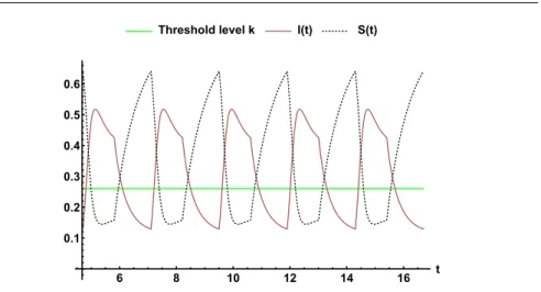
Fig. 6: The periodic solution for k= 0.26,γ = 1.38,β= 15.8,µ= 1.3,R0= 5.9, τ= 1,u∗= 0.76.

Note that it is possible to satisfy both inequalities (19) and (20) at the same time: for example, ifβ= 15, µ= 0.4, γ= 1 andu∗= 0.5, then both (19) and (20) hold.

Also observe that conditionk∈(0, k1) implies (C.3). Therefore Proposition 1 already guarantees thatE₂^∗is the unique endemic equilibrium for (Sys_d). For the second coordinate ofE^∗₁, we haveI₁^∗≥k.

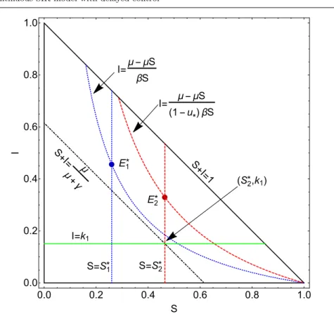
Fig. 8 explains the geometrical position of the segment I=k₁. Set

∆2=

(S, I)∈∆:S+I≥ µ µ+γ

.

It is straightforward to check that bothE^∗₁ andE^∗₂ belong to∆2.

We need the forthcoming two results before proving Theorem 4. First we show that all solutions of (Sysd) leave∆\∆2in finite time. Then we verify the positive invariance of∆2 independently of the choice of parameters.

Proposition 7 Assume (19) and suppose that (S(0), I(0)) ∈ ∆\∆2 for a solution (S, I)of(Sysd). Then there exists t0>0such that(S(t0), I(t0))∈∆2.

Proof First we claim that if (19) holds, then S_f⁰ andSc⁰ are both positive on the closure

∆\∆2=

(S, I)∈∆:I≤ µ µ+γ−S

of∆\∆2. Recall from Fig. 4 in Section 7 thatS_f⁰ andS_c⁰ are both positive on the subset

(S, I)∈∆:I <µ−µS βS

.

Hence it suffices to show that µ

µ+γ −S <µ−µS

βS for 0≤S≤ µ µ+γ.

(20)

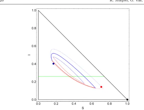
Fig. 7: The dashed, solid and dotted curves represent the periodic solution for τ= 0.4,1,4 respectively. The parameters arek= 0.26,γ= 1.38,β= 15.8,µ= 1.3, R0= 5.9,u∗= 0.76.

We investigate this inequality in the form µ

µ+γ +^µ

β < S+ ^µ

βS for all 0≤S≤1. (21)

The left-hand side is independent ofS. Examining the derivative of the right-hand side, it is easy to see that the right-hand side is minimal forS = p

µ/β, and it takes the value

S+ ^µ βS = 2

rµ

β forS=

rµ β.

We see from assumption (19) that inequality (21) holds for S = p

µ/β. Thus it holds for allS∈[0,1]. The proof of the claim is complete.

Let Mf and Mc be the minimum of S_f⁰ and Sc⁰ on ∆\∆2, respectively. As S_f⁰ and Sc⁰ are both continuous and positive on the compact subset ∆\∆2, the constantsM_f andMc are well-defined and positive.