Energy Distribution of a Vehicle Shimmy System with the Delayed Tyre Model ?
Tian Mi∗ Nan Chen∗ Gabor Stepan∗∗ Denes Takacs∗∗∗
∗School of Mechanical Engineering, Southeast University, Nanjing, China (e-mail: mitian@seu.edu.cn; nchen@seu.edu.cn).
∗∗Department of Applied Mechanics, Budapest University of Technology and Economics, Budapest, Hungary (e-mail:
stepan@mm.bme.hu).
∗∗∗MTA-BME Research Group on Dynamics of Machines and Vehicles, Budapest, Hungary (e-mail: takacs@mm.bme.hu).
Abstract: A vehicle shimmy model using the Delayed Tyre Model to estimate the lateral tyre force is introduced. Stability charts are obtained for the linearized system. With reduced damping and stiffness parameters, a new vibration mode shows up at high speed range when the front wheels oscillate in opposite directions. Furthermore, the kinetic energy distributed on each generalized coordinate is calculated at the critical frequencies, and some suggestions are given on how to reduce shimmy in specific cases.
Keywords:vehicle shimmy, Delayed Tyre Model, dynamic modeling, stability chart, energy distribution
1. INTRODUCTION
Vehicle shimmy, also known as ”death wobble”, is a self-excited vibration of the front wheels around their kingpins. It increases tyre wear, and deteriorates vehicle manoeuvrability.
A series of single wheel shimmy models corresponding to the aircraft landing gear or the trailer problems, have been studied by many researchers. Pacejka (2002) and Ran et al. (2014) use these shimmy models of different levels of complexity, determine the energy flow in the motion with the energy flow method, and compare different tyre models on shimmy. Much analytical and experimental work has been done on the shimmy of a trailer by using the Delayed Tyre Model in Takacs et al. (2009) and Takacs and Stepan (2012).
There is another type of shimmy models corresponding to the ground vehicles. In order to distinguish them from the single wheel models, ”vehicle shimmy” is used in this case. Vehicle shimmy models are often built with higher degrees of freedom (DoF), and take into account of the steering and suspension systems. Nonlinearities such as the tyre elasticity, dry friction, and clearance (or freeplay) of the steering system can all be considered. The semi- empirical tyre model – Pacejka’s Magic Formula (Pacejka, 2002) is widely used in vehicle shimmy problems, not only for the huge amounts of experimental validation of the tyre model, but also because that the nonlinearity can be introduced into the system in an explicit way, and the resultant ordinary differential equations are relatively easy
? This research was support by the National Natural Science Foun- dation of China (number: 51375086) and the China Scholarship Council.
to solve. For the related models, we refer to Li and Lin (2006), Wei et al. (2015) and Mi et al. (2017).
In this study, a 3 DoF vehicle shimmy model based on Li and Lin (2006) is established along with the Delayed Tyre Model as in Takacs et al. (2009). With the dependent sus- pension and the simplified steering system, the analytically more accurate tyre model can also be integrated without making the equations too lengthy.
The controller considering shimmy is difficult to design (see Goodwine and Stepan (2000)). In this respect, under- standing more about the vibration is of great importance.
If we can determine which part of the mechanism influ- ences shimmy the most, and make efforts to attenuate the vibration accordingly, it can be expected that the problem will be easier to deal with. This inspires us to check the energy distribution and to find out the specific parameters which may be used on shimmy control.
The rest of this paper is organized as follows: the dynamic model of the system and the tyre model are explained in section 2; in section 3, the stability charts and the corre- sponding frequency maps are obtained with the linearized system; the kinetic energy distributions in the generalized coordinates are calculated with different critical frequen- cies in section 4; finally, conclusions are given in section 5.
2. PROBLEM FORMULATION 2.1 System Modeling
With the assumptions that:
i) the vehicle runs at constant speed on a flat road, ii) the steering wheel is fixed,
ϕ ϕ ϕ
θ1 θ2
ce ce
Z
Y X
r l
vehicle body kingpin
kingpin k3
c3
k3
c3
k1 c1
k2 c2
γ γ
m v m
R
kz
kz
Fig. 1. Mechanical model.
iii) no longitudinal slip occurs between the tyre and road, a 3 DoF vehicle shimmy model (according to Li and Lin (2006)) is introduced in this section, where the vibrations of the left wheel θ1(t) and right wheel θ2(t) around their kingpins, and the swingϕ(t) of the dependent suspension about the longitudinal axis are all taken into account, see Fig. 1.
The equations of motion are given by:
(Jd+mr2) ¨θ1(t)−(Jd+1
2mlr) ¨ϕ(t) + (c1+c2+ +ce) ˙θ1(t)−c1θ˙2(t) +J0
v
Rϕ(t) + (k˙ 1+k2)θ1(t)−
−k1θ2(t)−1
2kzlrγ ϕ(t) =Q1, (Jd+mr2) ¨θ2(t)−(Jd+1
2mlr) ¨ϕ(t)−c1θ˙1(t)+
+ (c1+ce) ˙θ2(t) +J0
v
Rϕ(t)˙ −k1θ1(t) +k1θ2(t)−
−1
2kzlrγ ϕ(t) =Q2,
−(Jd+1
2mlr)γθ¨1(t)−(Jd+1
2mlr)γθ¨2(t) + (2Jd+ +1
2ml2) ¨ϕ(t)−J0
v
Rθ˙1(t)−J0
v
Rθ˙2(t) +c3ϕ(t)−˙
−1
2kzlrγ θ1(t)−1
2kzlrγ θ2(t) + (k3+1
2kzl2)ϕ(t) =Q3, (1) where Q1, Q2, and Q3 are the generalized forces; J0, Jd
are the mass moments of inertia of a wheel with respect to (w.r.t.) the rolling axle and its diameter, respectively;
c1,2,3,e and k1,2,3,z are damping and stiffness parameters, respectively;Ris the rolling radius of the wheel,mis the wheel mass, and γis the caster angle; see Fig. 1.
2.2 The Delayed Tyre Model
As shown in Fig. 2, the tyre is considered to be thin, thus the contact area decays into a line. Taking the left wheel as an example, the lateral tyre deformation is denoted by q1(x, t). In the (x, y) plane, L (a, q1(a, t)) is the leading point, R (−a, q1(−a, t)) is the rear point, and P (x, q1(x, t)) is an arbitrary point on the contact line,
where ais half of the contact length. With the stretched string-type tyre assumption (Takacs et al., 2009), the tyre deformation within the contact region is not restricted, and outside the contact area decays exponentially. The position of point P is expressed as
q1(x, t) =
q1(−a, t)e(x+a)/σ, ifx∈(−∞,−a);
q1(x, t), ifx∈[−a, a];
q1(a, t)e−(x−a)/σ, ifx∈(a,∞);
(2)
where σ is the relaxation length. The generalized forces are then given by
Q1,2=k Z ∞
−∞
(a−Rγ)q1,2(x, t)dx, Q3=
k Z ∞
−∞
q1(x, t)dx+k Z ∞
−∞
q2(x, t)dx R,
(3)
where k is the lateral tyre stiffness, and q2(x, t) is the lateral deformation of the right tyre.
y x
z
R
P L
a a σ x σ
R
y
P L
a a Tyre Contact Area
Fig. 2. Stretched string-type tyre.
In a coordinate system (X, Y, Z) fixed on the ground (see Fig. 1), the position of the tyre contact point can be derived by the matrix transformations. The linearized forms of the position vector in X and Y directions are given by
X(x, t) =vt−rθ1(t) +x, Y(x, t) = l
2 +q1(x, t) + (x−Rγ)θ1(t) +Rϕ(t). (4) With assumption iii), the tyre particles stick to the ground in the contact patch, that is,
dX
dt = 0, dY
dt = 0. (5)
The substitution of (4) into (5) leads to the expressions of
˙
xand dq1(x, t)/dt. The travelling wave solution is:
X(x, t) =X(a, t−τ), Y(x, t) =Y(a, t−τ), (6) where the delay τ is the time needed for the tyre particle to move from the leading point L to an arbitrary pointP on the contact line.
With dq1(x, t)/dt = ∂q1(x, t)/∂t+ ˙x·∂q1(x, t)/∂x and
∂q1(a, t)/∂x=−q(a, t)/σat the leading point P, equations (2)-(6) together with (1) give a system which will finally be governed by 3 delay differential equations (DDE) and two ordinary differential equations (ODE).
Note that the ideas are only explained in brief here, for details of the derivation we refer to Takacs et al. (2009) and Mi et al. (2017).
3. STABILITY ANALYSIS
For our system which contains DDEs, there are infinite many eigenvalues, but only a few of them locate in the right half of the complex plane. When the eigenvalues are in the imaginary axis, shimmy can occur in the corresponding nonlinear system. The stability boundary can be obtained by calculating the critical eigenvalues with certain parameter combinations.
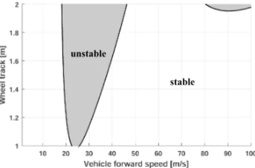
Fig. 3. Stability chart with realistic parameters.
Fixing the vehicle forward speedv and the wheel track l, stability chart for a heavy vehicle (Li and Lin, 2006) is shown in Fig. 3, and the parameters are given in Table.
1. Numerical method – the Bisection Method (Bachrathy and Stepan, 2012) is used due to the high dimension of the system.
In Fig. 3, there are two lobes in the speed ranges of 20- 50 m/s and 80-100 m/s, respectively, and the lobe in the larger speed range only shows up a little with very large wheel track though. To investigate more dynamic behaviours, we reduce the damping values c1,2,e in the steering system and at the kingpins by 0.4, and stiffness values k1,2 of the steering system by 0.7. The stability chart and the corresponding critical frequency map are
Fig. 4. Stability chart and the corresponding critical fre- quency map with reduced damping and stiffness of the steering system (and at the kingpins).
shown in Fig. 4, where more complicated vibrations occur.
The previously existing two lobes (similar as that in Fig.
3, with frequencies of 5-7 Hz and 10-15 Hz, respectively) come down and their boundaries cross each other, where the quasi-periodic oscillation is expected. A new lobe at very high speed (>65 m/s) with frequencies of about 15- 16 Hz shows up.
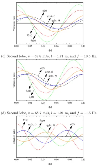
The vibration modes of the three selected points (marked with red circles) in Fig. 4 are shown in Fig. 5. Panel (a) is obtained at the pointv= 11.3 m/s,l= 1.50 m in the first lobe (with the lowest frequency of 5-7 Hz), with a critical frequency of 4.4 Hz. Panel (b) and (c) are obtained at the intersection pointv= 59.8 m/s,l= 1.71 m of the first lobe and second lobe (with the critical frequency of 10-15 Hz), and the frequencies are 6.5 Hz and 10.5 Hz, respectively.
Panel (d) and (e) are for the intersection point v = 68.7 m/s, l = 1.21 m of the second lobe and third lobe (with the highest frequency of 15-16 Hz), and the frequencies at different lobes are 11.5 Hz and 15.3 Hz, respectively.
Θ1HtL Θ2HtL q1Ha,tL
q2Ha,tL
jHtL
0.00 0.05 0.10 0.15 0.20 0.25 0.30
t@sD
Vibrationratio
(a) First lobe,v= 11.3 m/s,l= 1.50 m, andf= 4.4 Hz.
Θ1HtL Θ2HtL jHtL
q1Ha,tL q2Ha,tL
0.00 0.05 0.10 0.15 0.20
t@sD
Vibrationratio
(b) First lobe,v= 59.8 m/s,l= 1.71 m, andf= 6.5 Hz.
jHtL q1Ha,tL
q2Ha,tL
Θ1HtL Θ2HtL
0.00 0.02 0.04 0.06 0.08 0.10
t@sD
Vibrationratio
(c) Second lobe,v= 59.8 m/s,l= 1.71 m, andf= 10.5 Hz.
jHtL
Θ1HtL Θ2HtL
q1Ha,tL q2Ha,tL
0.00 0.02 0.04 0.06 0.08 0.10
t@sD
Vibrationratio
(d) Second lobe,v= 68.7 m/s,l= 1.21 m, andf= 11.5 Hz.
Θ1HtL Θ2HtL
jHtL q1Ha,tL q2Ha,tL
0.00 0.02 0.04 0.06 0.08 0.10
t@sD
Vibrationratio
(e) Third lobe,v= 68.7 m/s,l= 1.21 m, andf= 15.3 Hz.
Fig. 5. Vibration modes of the selected points in Fig. 4 with different frequencies.
In the first lobe corresponding to panel (a) and (b), the vibration amplitude of the swing angleϕ(t) is small, while the shimmy angles of front wheelsθ1,2(t) are much larger.
The tiny difference in the amplitudes between left and right wheels is caused by the asymmetry of the system, as depicted in Fig. 1. Compared with panel (a), the vibration amplitude of the swing angle ϕ(t) is larger in panel (b), and the phases of θ1,2(t) and ϕ(t) are shifted relative to the lateral tyre deformationsq1,2(a, t). It can be related to the wide speed range of the lobe. If we trace the vibration modes along the first lobe with realistic parameters in Fig.
3, the phases shift little by little with the increase of the speed, and so does the amplitude increase of ϕ(t). Panel (b) and (c) have very similar vibration modes, where the swing angleϕ(t) of the suspension vibrates more strongly compared with that in panel (a) and (b).
For the first two lobes, the contact linesq1(a, t) andq2(a, t) (or the shimmy angles θ1(t) and θ2(t)) are in the same phase, when the left and right wheels vibrate in the same direction. However, in panel (e) of Fig. 5, the front wheels vibrate in opposite phases.
4. ENERGY DISTRIBUTION
In order to investigate more details of the vibrations, the kinetic energy distributed in each generalized coordinate at different parameter combinations is checked in this part.
The energy of the system are also considered in Pacejka (2002) and Ran et al. (2014) , and the energy flow method is used to compare different tyre models, and to show how the energy flows from different input sources. On contrast, we do not focus on where the energy comes from, but on how it reflects on different coordinates.
The contribution of theith generalized coordinate to the total kinetic energy (see Shi et al. (2009)) can be calculated as
ηi(t) =Ti(t) T(t) =
3
P
j=1
Jijqi(t)qj(t)
3
P
i=1 3
P
j=1
Jijqi(t)qj(t)
×100%, i= 1,2,3,
(7) where Ti(t) is the kinetic energy distributed in ith gen- eralized coordinate (i.e. θ1(t),θ2(t), and ϕ(t)), Jij is the element of matrixJ inith row,jth column.
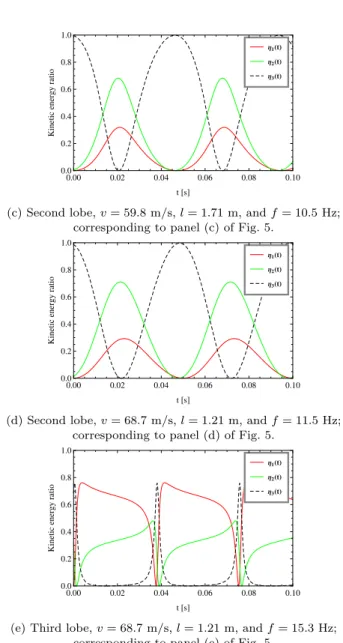
By calculating the eigenvectors of the critical eigenvalues, and substituting them into (7), the energy distributions corresponding to Fig. 5, panel (a)-(e) are pictured in Fig.
6, panel (a)-(e), respectively. Panel (a) and (b) in Fig. 6 show that, the proportion of the front-wheel vibrations is large in the first lobe, although that of the swing angle rises with the increase of the critical frequency. For the second lobe, the vibration of the suspension around the longitudinal axis increases dramatically, see panel (c) and (d). When the third lobe (see panel (e)) constitute the majority of the total energy, just like the first lobe.
Η1HtL Η2HtL Η3HtL
0.00 0.05 0.10 0.15 0.20 0.25 0.30
0.0 0.2 0.4 0.6 0.8 1.0
t@sD
Kineticenergyratio
(a) First lobe,v= 11.3 m/s,l= 1.50 m, andf= 4.4 Hz;
corresponding to panel (a) of Fig. 5.
Η1HtL Η2HtL Η3HtL
0.00 0.05 0.10 0.15 0.20
0.0 0.2 0.4 0.6 0.8 1.0
t@sD
Kineticenergyratio
(b) First lobe,v= 59.8 m/s,l= 1.71 m, andf= 6.5 Hz;
corresponding to panel (b) of Fig. 5.
Η1HtL Η2HtL Η3HtL
0.00 0.02 0.04 0.06 0.08 0.10
0.0 0.2 0.4 0.6 0.8 1.0
t@sD
Kineticenergyratio
(c) Second lobe,v= 59.8 m/s,l= 1.71 m, andf= 10.5 Hz;
corresponding to panel (c) of Fig. 5.
Η1HtL Η2HtL Η3HtL
0.00 0.02 0.04 0.06 0.08 0.10
0.0 0.2 0.4 0.6 0.8 1.0
t@sD
Kineticenergyratio
(d) Second lobe,v= 68.7 m/s,l= 1.21 m, andf= 11.5 Hz;
corresponding to panel (d) of Fig. 5.
Η1HtL Η2HtL Η3HtL
0.00 0.02 0.04 0.06 0.08 0.10
0.0 0.2 0.4 0.6 0.8 1.0
t@sD
Kineticenergyratio
(e) Third lobe,v= 68.7 m/s,l= 1.21 m, andf= 15.3 Hz;
corresponding to panel (e) of Fig. 5.
Fig. 6. Energy distributions on gereralized coordinates in different vibration modes corresponding to Fig. 5.
Now it will be interesting to see what happens if some specific damping values in different parts of the system are changed.
When the damping values corresponding to the front- wheel shimmy, that is,c1,2of the steering system or ce at the kingpins are increased while all the others remain the same with that in Fig. 4, the resulting stability charts and corresponding frequency maps are shown in Fig. 7. Either we increasec1,2(see panel (a) of Fig. 7) orce(see panel (b) of Fig. 7) by a factor of 1.5, the third lobe disappears in the shown region. Compared to the stability chart in Fig.
4, the first two lobes almost stand in the same positions – they become a bit smaller indeed but not palpable. It agrees with the energy distribution in panel (e) of Fig. 6.
The stability chart and frequency map with increased dampingc3of the suspension around longitudinal axis are shown in Fig. 8, where the damping is multiplied by a factor of 1.5 also. This time, the first lobe and third lobe remain but the second lobe goes up.
(a)c1,2are increased by a factor of 1.5.
(b)ceis increased by a factor of 1.5.
Fig. 7. Stability charts obtained with increased damping values of the steering system and at the kingpins.
To conclude, the first lobe is ”stubborn”, and does not change much with the increase of specific damping value(s). When the total damping is increased, the first lobe goes up, and the unstable region becomes smaller (see Fig. 3). The second lobe is sensitive to the suspension damping (c3), and the third lobe is sensitive to the damp- ing parameters corresponding to the front-wheel shimmy (i.e.c1,2andce).
Fig. 8. Stability chart obtained with increased damping valuec3of the suspension around the longitudinal axis by a factor of 1.5.
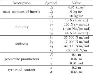
Table 1. Parameters in the stability analysis.
Description Symbol Value
mass moment of inertia
J0 4.85 kg m2
Jd 6 kg m2
J3 20 kg m2
damping
c1 10 N s/(m rad) c2 100 N s/(m rad) c3 1 050 N s/(m rad) ce 44 N s/(m rad)
stiffness
k1 35 500 N m/rad k2 17 000 N m/rad k3 32 000 N m/rad kz 400 000 N/m geometric parameters
R 0.4 m
r 0.07 m
γ 0.04 rad
tyre-road contact a 0.2 m
σ 0.65 m
5. CONCLUSION
In this paper, a 3 DoF shimmy model taking into account the steering system and the suspension system is intro- duced with the Delayed Tyre Model. Constraint equations are derived with the stretched string-type tyre assumption, which considers the lateral tyre deformation both in and out of the contact patch. The resultant system with delay differential equations is linearized and the stability charts are obtained by numerical method.
For more interesting dynamic behaviours of the system, the damping and stiffness values are reduced. As a result, quasi-periodic oscillations occur, and even a new lobe appears. By determining the eigenvectors corresponding to the critical frequencies at some chosen points in the stability chart, the vibration modes are visualized. It turns out that in the previous existing two lobes, the front wheels vibrate in the same direction, while in opposite phases in the new lobe.
By calculating the kinetic energy distribution in each gen- eralized coordinate, the main energy consuming coordi- nate(s) can be determined. If we increase the correspond- ing damping values of the components, the unstable lobes in the high speed range shrink dramatically. However, the lobe with lowest critical frequency stays still.
Although the vibration modes can already provide much information about shimmy, the differences among diverse modes are vague. If we further calculate the kinetic energy of each generalized coordinate, the results show that even the similar looking vibration modes (such as the first and second lobes) can have very different energy distributions, and the attenuation of shimmy can be related to different damping parameters.
With the development of the technology, the maximum speed of ground vehicles is increasing, and the control strategies have been developed in various driving condi- tions. But shimmy is rarely taken into account in the con- troller designing. This paper introduces a dynamic model considering steering and suspensions systems, and gives some analytical reference for vehicles, for example, with multiple active dampers, on how to deal with the shimmy problem.
The model is established with many simplifications and assumptions: some geometric parameters such as the cam- ber angle are not considered; the tyre contact length and the relaxation length are taken as constants; the steering wheel is fixed; the translational and rotational movements of many components are neglected, etc. The suggestions on shimmy attenuation are neither direct nor easily achiev- able, especially with a heavy truck at very high speed.
However, from the view point of understanding more about the shimmy phenomenon, this work can still provide some valuable reference in the future research.
ACKNOWLEDGEMENTS
This research was support by the National Natural Science Foundation of China (number: 51375086) and the China Scholarship Council.
REFERENCES
Bachrathy, D. and Stepan, G. (2012). Bisection method in higher dimensions and the efficiency number. Periodica Polytechnica Mechanical Engineering, 56(2), 81–86.
Goodwine, B. and Stepan, G. (2000). Controlling unstable rolling phenomena. Journal of Vibration and Control, 6(1), 137–158.
Li, S. and Lin, Y. (2006). Study on the bifurcation character of steering wheel self-excited shimmy of motor vehicle. Vehicle System Dynamics, 44(sup1), 115–128.
Mi, T., Stepan, G., Takacs, D., and Chen, N. (2017).
Shimmy model for electric vehicle with independent sus- pensions. Proceedings of the Institution of Mechanical Engineers Part D Journal of Automobile Engineering, (24), 095440701770128.
Pacejka, H.B. (2002). Tyre and vehicle dynamics.
Butterworth-Heinemann.
Ran, S., Besselink, I.J.M., and Nijmeijer, H. (2014). Ap- plication of nonlinear tyre models to analyse shimmy.
Vehicle System Dynamics, 52(sup1), 387–404.
Shi, W.K., Fu, J.H., Hao, Y., and Teng, T. (2009). Multi- objective optimization of powertrain mounting based on matlab. In Computational Intelligence and Industrial Applications, 2009. PACIIA 2009. Asia-Pacific Confer- ence on, 484–487.
Takacs, D., Orosz, G., and Stepan, G. (2009). Delay effects in shimmy dynamics of wheels with stretched string-like tyres.European Journal of Mechanics / A Solids, 28(3), 516–525.
Takacs, D. and Stepan, G. (2012). Micro-shimmy of towed structures in experimentally uncharted unstable parameter domain. Vehicle System Dynamics, 50(11), 1613–1630.
Wei, D., Xu, K., Jiang, Y., Chen, C., Zhao, W., and Zhou, F. (2015). Hopf bifurcation characteristics of dual-front axle self-excited shimmy system for heavy truck consid- ering dry friction. Shock and Vibration,2015,(2015-12- 8), 2015(1), 1–20.