Planar S-systems: Global stability and the center problem

Planar S-systems:

Global stability and the center problem

Bal´ azs Boros, Josef Hofbauer, Stefan M¨ uller

, Georg Regensburger

May 9, 2018

Abstract

S-systems are simple examples of power-law dynamical systems (polyno- mial systems with real exponents). For planar S-systems, we study global stability of the unique positive equilibrium and solve the center problem.

Further, we construct a planar S-system with two limit cycles.

Keywords: power-law systems, center-focus problem, first integrals, re- versible systems, focal values, global centers, limit cycles, Andronov-Hopf bifurcation, Bautin bifurcation

AMS subject classification: 34C05, 34C07, 34C14, 34C23, 80A30, 92C42

1 Introduction

An S-system is a dynamical system on the positive orthant for which the right hand side is given bybinomials(differences of monomials) with real exponents.

S-systems were introduced by Savageau [12, 13] in the context of biochemical systems theory. For a recent review and an extensive list of references, see [16].

In biochemical systems theory, one also considers dynamical systems given by polynomialswith real exponents (power-law systems).

As already observed in [13], the binomial structure of an S-system allows to reduce the computation of positive equilibria to linear algebra by taking the logarithm. In particular, it is easy to characterize when such a dynamical system has a unique positive equilibrium. At the same time, already aplanarS-system with a unique positive equilibrium may give rise to rich dynamical behaviour, as demonstrated in this paper.

Bal´azs Boros·Josef Hofbauer·Stefan M¨uller

Department of Mathematics, University of Vienna, Oskar-Morgenstern-Platz 1, 1090 Wien, Austria Georg Regensburger

Institute for Algebra, Johannes Kepler University Linz, Altenbergerstrasse 69, 4040 Linz, Austria

∗Corresponding author st.mueller@univie.ac.at

arXiv:1707.02104v2 [math.DS] 8 May 2018

Andronov-Hopf bifurcations of planar S-systems are discussed in [7], and the first focal value is used to construct a stable limit cycle in [17]. In fact, the first mathematical model of glycolytic oscillations by Selkov [14] is a planar S-system.

In previous work, we studied planar S-systems arising from a chemical reaction network (the Lotka reactions) with power-law kinetics. A global stability analy- sis is given in [1], and the center problem is solved in [2]. (For an interpretation of S-systems as dynamical systems arising from chemical reaction networks with generalized mass-action kinetics [9], we refer the reader to Appendix A.) In this paper, we provide a global stability analysis of arbitrary planar S-systems (Section 3). In particular, we characterize the real exponents for which the unique equilibrium of a planar S-system is globally stable for all positive coeffi- cients. Further, we determine the parameters for which the unique equilibrium is a center (Section 4). In particular, we characterize global centers (Subsec- tion 4.5), and finally we construct a planar S-system with two limit cycles bi- furcating from a center (Subsection 4.6). It remains open whether there exist planar S-systems with more than two limit cycles, and we discuss a “fewnomial version” of Hilbert’s 16th problem asking for an upper bound on the number of limit cycles for planar power-law systems in terms of the number of monomials.

For an illustration of our analysis, we provide figures in Appendix B.

In the following section, we introduce planar S-systems, bring them into expo- nential form, and discuss the resulting symmetries.

2 Planar S-systems

A planar S-system is given by

˙

x1=α1x^g₁¹¹x^g₂¹²−β1x^h₁¹¹x^h₂¹², (1)

˙

x2=α2x^g₁²¹x^g₂²²−β2x^h₁²¹x^h₂²²

with α1, α2, β1, β2 ∈ R+ and g11, g12, g21, g22, h11, h12, h21, h22 ∈ R. Since we allow real exponents, we study the dynamics on the positive quadrantR²+. We assume that the ODE (1) admits a positive equilibrium (x^∗₁, x^∗₂), and use the equilibrium to scale the ODE. We obtain

˙ x1=γ1

x^g₁¹¹x^g₂¹²−x^h₁¹¹x^h₂¹²

, (2)

˙

x₂=γ₂

x^g₁²¹x^g₂²²−x^h₁²¹x^h₂²² ,

where γ1 = α1(x^∗₁)^g11−1(x^∗₂)^g12 and γ2 = α2(x^∗₁)^g21(x^∗₂)^g22−1. The ODE (2) admits the equilibrium (1,1).

By a nonlinear transformation, we obtain a planar system with the origin as the unique equilibrium. In this exponential form, nullclines are straight lines and symmetries in the exponents can be exploited.

2.1 Exponential form

Given the ODE (2), we perform the nonlinear transformations x1= e^γ1u and x2= e^γ2v

and obtain

˙

u= e^a1u+b1v−e^a2u+b2v, (3)

˙

v= e^a3u+b3v−e^a4u+b4v, defined onR², where

a1=γ1(g11−1), b1=γ2g12, (4) a₂=γ₁(h₁₁−1), b₂=γ₂h₁₂,

a3=γ1g21, b3=γ2(g22−1), a₄=γ₁h₂₁, b₄=γ₂(h₂₂−1).

The ODE (3) admits the equilibrium (0,0), and the Jacobian matrix at (0,0) is given by

J =

a1−a2 b1−b2

a3−a4 b3−b4

. (5)

We abbreviate the ODE (3) by its 8 parameters, more specifically, by the scheme a₁ a₂ a₃ a₄

b₁ b₂ b₃ b₄

. (6)

For anya, b∈R, the ODE abbreviated by the parameter scheme a₁−a a₂−a a₃−a a₄−a

b1−b b2−b b3−b b4−b

is obtained by multiplying the vector field in the ODE (3) with e^−au−bv and is hence orbitally equivalent to (3). Thus the number of parameters could be reduced from 8 to 6.

Applying a uniform scaling transformation (u, v) 7→ (cu, cv) with c > 0 and rescaling time accordingly is equivalent to dividing all parameters byc. Hence, the parameter space could be reduced to a 5-dimensional compact manifold.

2.2 Symmetry operations

In the proofs of our main results (Sections 3 and 4), we exploit symmetries in the parameters, in order to avoid tedious case distinctions.

In fact, the family of ODEs (3) is invariant under the symmetry group of the square (the dihedral group D4) which consists of the following eight elements (rotations and reflections inR²):

r₀= 1 0

0 1

, r₁=

0 −1

1 0

, r₂=

−1 0 0 −1

, r₃=

0 1

−1 0

,

s₀=

1 0 0 −1

, s₁= 0 1

1 0

, s₂=

−1 0 0 1

, s₃=

0 −1

−1 0

.

The question arises how these symmetry operations transform the ODE (3). We start withr₁, the rotation by 90^◦. For (U, V) =r₁(u, v), that is,U =−v, V =u, we obtain

U˙ =−v˙= e^a4u+b4v−e^a3u+b3v = e^−b4U+a4V −e^−b3U+a3V, V˙ = ˙u = e^a1u+b1v−e^a2u+b2v = e^−b1U+a1V −e^−b2U+a2V .

Sor1 transforms the ODE (3), abbreviated by the parameter scheme (6), into the ODE abbreviated by

−b₄ −b₃ −b₁ −b₂ a4 a3 a1 a2

. (7)

The other operations transform the parameter scheme (6) as follows:

r2:

−a2 −a1 −a4 −a3

−b2 −b1 −b4 −b3

(8)

r₃:

b₃ b₄ b₂ b₁

−a₃ −a₄ −a₂ −a₁

(9)

s0:

a1 a2 a4 a3

−b1 −b2 −b4 −b3

(10)

s1:

b3 b4 b1 b2

a3 a4 a1 a2

(11)

s₂:

−a2 −a1 −a3 −a4

b₂ b₁ b₃ b₄

(12)

s₃:

−b4 −b3 −b2 −b1

−a4 −a3 −a2 −a1

(13) Note that the symmetry operations r₀,r₂,s₀,s₂ keep the roles of a_i and b_i (as coefficients of u and v, respectively), whereas the other four operations interchange them. Only the subgroup consisting of r₀,s₁ keeps the signs of botha_i andb_i.

Finally, the time reversalt7→ −ttransforms (3) into a2 a1 a4 a3

b2 b1 b4 b3

. (14)

3 Global stability

Ultimately, we are interested in stability properties of the unique positive equi- librium of the ODE (1). LetG= (g_ij)∈R^2×2and H = (h_ij)∈R^2×2. A short calculation shows that the condition

det(G−H)6= 0

ensures that the ODE (1) admits a unique positive equilibrium for all given values of the positive parameters α₁, α₂, β₁, β₂. Then (1,1) is the unique positive equilibrium of the ODE (2), and (0,0) is the unique equilibrium of the ODE (3) with (4). On the other hand, if det(G−H) = 0, then the ODE (1) admits either no equilibrium or infinitely many equilibria, depending on the specific values ofα1,α2,β1,β2.

We call an equilibrium (inR²+) of the ODEs (1) or (2) or an equilibrium (inR²) of the ODE (3) with (4) globally asymptotically stable if it is Lyapunov stable and from each initial condition the solution converges to the equilibrium.

Below, we characterize the parametersGandH (the real exponents) for which the resulting ODEs admit a unique equilibrium that is (globally) asymptotically stable forall otherparameters (the positive coefficients). To begin with, we state the obvious relation between the stability properties of the ODEs (1), (2), and (3) with (4).

Proposition 1. FixG, H∈R^2×2withdet(G−H)6= 0. Then the following are equivalent:

(i) The unique positive equilibrium(x^∗₁, x^∗₂)of the ODE (1)is (globally) asymp- totically stable for all α₁, α₂, β₁, β₂>0.

(ii) The unique positive equilibrium(1,1) of the ODE (2) is (globally) asymp- totically stable for all γ1, γ2>0.

(iii) The unique equilibrium(0,0)of the ODE (3)with (4)is (globally) asymp- totically stable for all γ1, γ2>0.

In our main results, we consider the ODE (3) with (4) and write the Jacobian matrix (5) with (4) as

J = (G−H)

γ1 0 0 γ2

.

Clearly, signJ = sign(G−H) and sign(detJ) = sign(det(G−H)). In particular, detJ 6= 0 if and only if det(G−H) 6= 0. First, we characterize asymptotic stability.

Proposition 2. FixG, H∈R^2×2withdet(G−H)6= 0and letJbe the Jacobian matrix of the ODE (3)with (4)at the origin. Then the following are equivalent:

(i) The unique equilibrium (0,0) of the ODE (3) with (4) is asymptotically stable for allγ1, γ2>0.

(ii) detJ >0 andsignJ equals one of the sign matrices − ∗

∗ −

,

0 +

− −

,

0 −

+ −

,

− −

+ 0

,

− +

− 0

.

In particular, these conditions are independent of γ1, γ2>0.

Proof. Statement (ii) implies detJ >0 and trJ <0, and statement (i) follows by a theorem of Lyapunov. By the same theorem (together with the assumption detJ 6= 0), statement (i) implies detJ >0 and trJ ≤0 for allγ1, γ2>0. The

trace condition is equivalent to both diagonal entries of J being non-positive.

However, both diagonal entries being zero makes the origin a center, as can be seen using the integrating factor e^−a1u−b4v, cf. case S in Subsection 4.1. The signs of the off-diagonal entries follow from detJ >0.

In our main result, we characterize global stability.

Theorem 3. Fix G, H∈R^2×2 with det(G−H)6= 0 and letJ be the Jacobian matrix of the ODE (3)with (4)at the origin. Then the following are equivalent:

(i) The unique equilibrium (0,0) of the ODE (3) with (4) is globally asymp- totically stable for all γ1, γ2>0.

(ii) detJ >0 and either (a) signJ =

− ∗

∗ −

, (b) signJ =

0 +

− −

anda₃≤a₁=a₂≤a₄, (c) signJ =

0 −

+ −

anda₄≤a₁=a₂≤a₃, (d) signJ =

− −

+ 0

andb1≤b3=b4≤b2, or (e) signJ =

− +

− 0

andb2≤b3=b4≤b1.

In particular, these conditions are independent of γ₁, γ₂>0.

The proof of Theorem 3 requires two auxiliary results, Lemmas 4 and 5. There we study the ODE (3) without the substitutions (4). Recall that its Jacobian matrix is given by (5), that is,

J =

a1−a2 b1−b2

a3−a4 b3−b4

.

Lemma 4 on the non-existence of periodic solutions will also be useful in Sub- section 4.1, where we look for first integrals of the ODE (3). Lemma 5 on the boundedness of solutions will also be useful in Subsection 4.5, where we solve the global center problem.

Lemma 4. Let a1 ≤a2, b3 ≤b4 with (a1−a2, b3−b4)6= (0,0). Further, let a1≤a≤a2 andb3≤b≤b4. Then,

(a) the r.h.s. of the ODE (3)multiplied by e^−au−bv has negative divergence, (b) there is no periodic solution of the ODE (3).

Proof. Letf denote the r.h.s. of the ODE (3). Multiplyingf(u, v) byh(u, v) = e^−au−bv yields a vector field with negative divergence, since

div(hf)

h (u, v) = (a1−a) e^a1u+b1v+(a−a2) e^a2u+b2v + (b₃−b) e^a3u+b3v+(b−b₄) e^a4u+b4v. By the Bendixson-Dulac test, (a) implies (b).

Lemma 5. Let J be the Jacobian matrix of the ODE (3) at the origin with detJ > 0. The following statements provide conditions for the boundedness of all solutions of the ODE (3)in positive time.

(a) IfsignJ=

− ∗

∗ −

, then boundedness holds.

(b1) IfsignJ=

+ +

− −

, then boundedness implies a3≤a2< a1≤a4.

(b2) IfsignJ =

0 +

− −

, then boundedness is equivalent toa3≤a2=a1≤a4. (c1) IfsignJ=

+ −

+ −

, then boundedness implies a₄≤a₂< a₁≤a₃.

(c2) IfsignJ =

0 −

+ −

, then boundedness is equivalent toa4≤a2=a1≤a3. (d1) IfsignJ=

− −

+ +

, then boundedness implies b1≤b4< b3≤b2.

(d2) IfsignJ =

− −

+ 0

, then boundedness is equivalent tob₁≤b₄=b₃≤b₂.

(e1) IfsignJ=

− +

− +

, then boundedness implies b2≤b4< b3≤b1.

(e2) IfsignJ =

− +

− 0

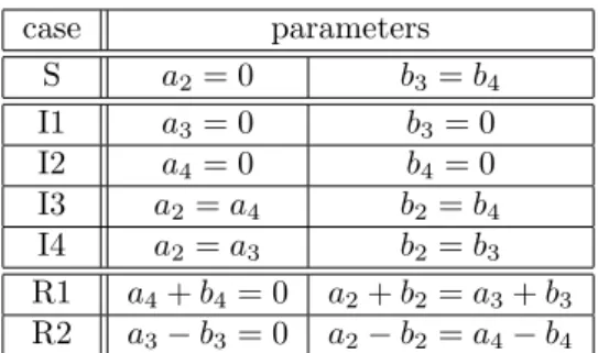
, then boundedness is equivalent tob2≤b4=b3≤b1. Proof. We start by proving (a). In order to prove the boundedness of the solutions in the case a₁ < a₂, b₃ < b₄, and detJ >0, we consider all possible signs ofa3−a4andb1−b2and the corresponding nullcline geometries. For phase portraits in the nine cases, see Figure 1. In two cases (top left and bottom right), solutions may spiral around the origin. Since the divergence of a scaled version of the right-hand side of the ODE (3) is negative (see Lemma 4), they can spiral inwards only (anti-clockwise and clockwise, respectively). In the other seven cases, two of the four regions bounded by the nullclines are forward invariant, hence solutions are ultimately monotonic in both coordinates and converge to the origin.

The symmetry operations (of the square) introduced in Subsection 2.2 preserve detJ > 0 and the boundedness of solutions. Hence, statements (c), (d), and (e) follow from (b) by applying the operations s0 ors2,s1 or s3, andr1 or r3, respectively, and it suffices to prove (b).

(b)

r₀,r₂

_s0,s2 //

r₁,r₃

s₁,s₃

(c)

(e) (d)

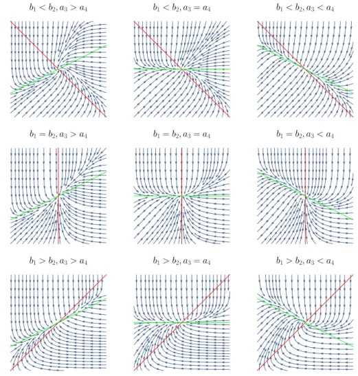
To prove (b1), first note that a₃ ≤ a₂ follows from a₁ ≤ a₄ by applying the operation r₂. Since a₂ < a₁ follows from the definition of the sign matrix, it suffices to prove thata₁≤a₄is necessary for the boundedness. Assumea₁> a₄ anda1> a2. A short calculation shows that the set

{(u, v)∈R² |u≥u0 andγu≤v≤γu0}

is forward invariant under the ODE (3) ifγ <0,|γ|is small enough, andu0>0 is large enough. All the solutions starting in this forward invariant set are monotonic in both coordinates and unbounded. For an illustration, see the top panel in Figure 2.

We now show the necessity of a3 ≤a2 =a1 ≤a4 for the boundedness in (b2).

The same argument as in the proof of (b1) shows that it suffices to prove that a1 ≤a4 is necessary for the boundedness. Assumea1 > a4 and a1 =a2 and consider the auxiliary ODE

˙

u= e^a1u+b1v−e^a2u+b2v, (15)

˙

v=−e^a4u+b4v,

which can be solved by separation of variables. Forv >0, the curve given by e^(b1−b4)v−1

b₁−b₄ −e^(b2−b4)v−1

b₂−b₄ =−e^(a4−a1)u

a₄−a₁ (16)

is an orbit of the ODE (15) with u→+∞,v →0 fort → ∞. All solutions of the ODE (3) that start above this curve are monotonic in both coordinates and unbounded. For an illustration, see the bottom panel in Figure 2. Ifb1−b4or b2−b4 is zero, replace ^eαv_α⁻¹ byv in (16).

It is left to show the sufficiency of a₃ ≤ a₂ = a₁ ≤ a₄ for the boundedness in (b2). One can use a Lyapunov function V : R² → R with (∂₁V)(u, v) =

−e^−a1u(e^a3u−e^a4u) and (∂₂V)(u, v) = e^−b4v(e^b1v−e^b2v). Assuming a₃ < a₄ andb1> b2 (recall the assumption on signJ), the boundedness of the sublevel sets of V is equivalent to a3 ≤ a1 ≤ a4 and b2 ≤ b4 ≤ b1, see Figure 3 for the illustration of the level sets of V. Thus, if in addition to a3 ≤ a1 ≤ a4, the inequalities b2≤b4≤b1also hold, the boundedness of the solutions of the ODE (3) follows. In case the inequalitiesb2≤b4≤b1do not hold, we also need to take into account the sign structure of the vector field in order to conclude the boundedness of the solutions. If b2≤b4b1, the set

{(u, v)∈R² |V(u, v)≤candv≤d}

is bounded and forward invariant for all c and for all sufficiently large d. If b₂b₄≤b₁, the set

{(u, v)∈R² |V(u, v)≤candv≥d}

is bounded and forward invariant for allcand for all sufficiently negatived. For an illustration of the constructed sets, see Figure 4.

Finally, we prove our main result.

Proof of Theorem 3. We have to show that among the systems fulfilling con- dition (ii) in Proposition 2 exactly those do not admit periodic or unbounded solutions that meet condition (ii) in the present theorem.

In fact, all systems fulfilling condition (ii) in Proposition 2 are covered by Lemma 4 and hence do not admit a periodic solution. Now, statements (a), (b2), (c2), (d2), (e2) in Lemma 5 characterize those systems that do not admit an unbounded solution.

4 The center problem

An equilibrium is a centerif all nearby orbits are closed.

Our aim is to characterize all parameters a1,a2,a3,a4,b1,b2, b3,b4 for which the origin is a center of the ODE (3). First, we look for first integrals, then we find centers of reversible systems, and indeed we prove that we have identified all possible centers. Thereby we use that an equilibrium (of an analytic ODE) is a center if and only if all focal values (Lyapunov coefficients) vanish, see [5, Chapters 3.5 and 8.3] or [11, Chapter 3.1].

Additionally, we characterize all the parameters for which the origin is aglobal center. Finally, we construct a system with two limit cycles.

Let J be the Jacobian matrix of the ODE (3) at the origin. For the origin to be a center, it is a prerequisite that trJ = 0 and detJ > 0. (If detJ = 0, then the origin lies on a curve of equilibria.) Hence, we assume these conditions throughout Subsections 4.1 and 4.2.

4.1 First integrals

We look for first integrals (constants of motion) for the ODE (3) and try an integrating factor of the forme^−au−bv. As we have seen in the proof of Lemma 4, the divergence is proportional to

(a1−a) e^a1u+b1v−(a2−a) e^a2u+b2v+(b3−b) e^a3u+b3v−(b4−b) e^a4u+b4v. (17) First, we consider

a1=a2andb3=b4. (case S)

Setting a=a₁ and b=b₄, all four terms vanish, and the system is integrable.

In fact, the ODE (3) is orbitally equivalent to

˙

u= e^(b1−b4)v−e^(b2−b4)v,

˙

v= e^(a3−a1)u−e^(a4−a1)u,

a system with separated variables. This case has codimension 2 in the parameter space.

Next, we consider

a1=a3and b1=b3. (case I1) The divergence (17) simplifies to

(a₁−a+b₃−b) e^a1u+b1v−(a2−a) e^a2u+b2v−(b4−b) e^a4u+b4v.

Setting a=a₂ andb=b₄, the last two terms vanish, and the first term is zero due to trJ = 0. This case has codimension 3 in the parameter space.

The following cases can be treated in the same way (and have codimension 3 in the parameter space):

a₁=a₄ andb₁=b₄ (case I2) a2=a4 andb2=b4 (case I3) a₂=a₃ andb₂=b₃ (case I4)

It is easy to see that case S is invariant under all symmetry operations.

On the other hand, cases I1–I4 can be obtained from each other by symmetry operations. Below, we apply all symmetry operations to case I1:

I1

r0,s1

r₃,s₀ //

r1,s2

r2,s3

I2

I4 I3

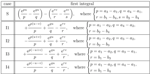
The corresponding first integrals are displayed in Table 1.

4.2 Reversible systems

LetR:R²→R²be a reflection along a line. A vector fieldF:R²→R²(and the resulting dynamical system) is called reversible w.r.t.RifF◦R=−R◦F. The following is a well-known fact, see e.g. [10, Chapter II, 4.6571], [11, Chapter 3.5], or more generally [3, Theorem 8.1]: an equilibrium of a reversible system which has purely imaginary eigenvalues and lies on the symmetry line ofRis a center.

The above definition can be generalized and the fact still holds: A vector field (system) F is reversible w.r.t. the reflection R if −R⁻¹◦F ◦R = λF with

case first integral S

e^pu p −e^qu

q

− e^rv

r −e^sv s

, where

(p=a₃−a₁, q=a₄−a₁, r=b1−b4, s=b2−b4

I1 +e^p(u−v) p +e^qu

q −e^rv

r , where

(p=a1−a2, q=a4−a2, r=b₂−b₄

I2 −e^p(u+v) p +e^qu

q +e^rv

r , where

(p=a₁−a₂, q=a₃−a₂, r=b2−b3

I3 +e^p(−u+v) p −e^qu

q +e^rv

r , where

(p=a1−a2, q=a3−a1, r=b₁−b₃

I4 −e^p(−u−v) p −e^qu

q −e^rv

r , where

(p=a1−a2, q=a4−a1, r=b1−b4

Table 1: First integrals corresponding to cases S, I1, I2, I3, I4. Ifαis zero in

e^αz

α (in a first integral), replace ^eαz_α byz.

λ:R² → R+. That is, if F transformed by R followed by time reversal is orbitally equivalent to F.

The ODE (3) is reversible w.r.t.s1, the reflection along the lineu= v, if the system transformed bys1followed by time reversal is orbitally equivalent to the original system. That is, if applying (14) to (11) is equivalent to the original scheme,

b₄ b₃ b₂ b₁ a₄ a₃ a₂ a₁

∼

a₁ a₂ a₃ a₄ b₁ b₂ b₃ b₄

.

This holds if and only if there exista, b∈Rsuch that a₁−a=b₄, b₁−b=a₄, a2−a=b3, b2−b=a3, a₃−a=b₂, b₃−b=a₂, a4−a=b1, b4−b=a1, that is,

a1−b4=a2−b3=a3−b2=a4−b1

or, equivalently,

a₁+b₁=a₄+b₄, a₂+b₂=a₃+b₃, and trJ = 0. (case R1) (18) The ODE (3) is reversible w.r.t. s₃, the reflection along the lineu=−v, if the system transformed bys₃followed by time reversal is orbitally equivalent to the original system. That is, if applying (14) to (13) is equivalent to the original scheme,

−b3 −b4 −b1 −b2

−a3 −a4 −a1 −a2

∼

a1 a2 a3 a4

b1 b2 b3 b4

.

This holds if and only if there exista, b∈Rsuch that a1−a=−b3, b1−b=−a3, a2−a=−b4, b2−b=−a4, a3−a=−b1, b3−b=−a1, a4−a=−b2, b4−b=−a2, that is,

a₁+b₃=a₂+b₄=a₃+b₁=a₄+b₂ or, equivalently,

a₁−b₁=a₃−b₃, a₂−b₂=a₄−b₄, and trJ = 0. (case R2) (19) The two families of reversible systems given by (18) and (19), respectively, have codimension 3 in the parameter space. The other two reflections, s0 and s2

(across the u- and v-axis), also lead to reversible systems, however, they are already covered by case S.

Cases R1 and R2 can be obtained from each other by symmetry operations.

Below, we apply all symmetry operations to case R1:

R1

r₀,r₂,s₁,s₃

_r1,r3,s0,s2 //R2

Finally, we remark that neither for R1 nor for R2 we were able to find a first integral. However, for systems that are in the intersection of R1 and R2, the functions

h

1 + e^r(u+v)i

[e^qu+ e^qv]^−rq and e^−a1u−b4v(e^qu+ e^qv)^−q+rq

serve as first integral and integrating factor, respectively, whereq=a4−a1and r=a3−a1.

4.3 Main result

In Table 2, we display the seven cases of centers we identified in Subsections 4.1 and 4.2. Indeed these are all possible centers of the ODE (3).

Theorem 6. Let J be the Jacobian matrix of the ODE (3) at the origin, that is,

J =

a1−a2 b1−b2

a3−a4 b3−b4

.

The following statements are equivalent:

1. The origin is a center of the ODE (3).

2. The eigenvalues of the Jacobian matrix at the origin are purely imaginary, that is,trJ = 0anddetJ >0, and the first two focal values vanish.

case parameters

S a1=a2 b3=b4

I1 a1=a3 b1=b3

I2 a1=a4 b1=b4

I3 a2=a4 b2=b4

I4 a2=a3 b2=b3

R1 a1+b1=a4+b4 a2+b2=a3+b3

R2 a₁−b₁=a₃−b₃ a₂−b₂=a₄−b₄

Table 2: Special cases of the ODE (3) having a center. Additionally, in all cases trJ = a₁−a₂+b₃−b₄ = 0, which is trivially fulfilled in case S, and detJ = (a₁−a₂)(b₃−b₄)−(a₃−a₄)(b₁−b₂)>0.

3. The parameter valuesa1,a2,a3,a4,b1,b2,b3,b4 belong to (at least) one of the seven cases S, I1, I2, I3, I4, R1, and R2 in Table 2.

Proof. 1⇒2: IfJ has a zero eigenvalue, that is, detJ = 0, then the origin lies on a curve of equilibria and cannot be a center. Hence, the eigenvalues ofJ are purely imaginary, and all focal values vanish.

2⇒3: For the computation of the first two focal values,L₁andL₂, and the case distinction implied by trJ = 0, detJ >0, andL₁=L₂= 0, see Subsection 4.4.

3⇒1: For the cases S, I1, I2, I3, and I4 in Table 2, we have found first integrals in Subsection 4.1. The remaining cases R1 and R2 are reversible systems, see Subsection 4.2.

4.4 Computation of focal values and case distinction

Instead of the ODE (3), we consider

˙

u= 1−e^a2u+b2v, (20)

˙

v= e^a3u+b3v−e^a4u+b4v. After performing the substitutions

a₂→a₂−a₁, b₂→b₂−b₁, (21) a3→a3−a1, b3→b3−b1,

a4→a4−a1, b4→b4−b1, the ODE (20) is orbitally equivalent to (3). Using

trJ =−a2+b3−b4= 0,

we compute detJ and the first two focal values,L1 andL2. We find detJ = (a3−a4)b2−(b3−b4)²

case parameters

S a2= 0 b3=b4

I1 a3= 0 b3= 0

I2 a4= 0 b4= 0

I3 a2=a4 b2=b4

I4 a2=a3 b2=b3

R1 a4+b4= 0 a2+b2=a3+b3

R2 a₃−b₃= 0 a₂−b₂=a₄−b₄

Table 3: Special cases of the ODE (20) having a center. Additionally, in all cases trJ =−a2+b₃−b₄= 0, which is trivially fulfilled in case S, and detJ = (a₃−a₄)b₂−(b₃−b₄)²>0.

and note that detJ >0 impliesa₃ 6=a₄ andb₂6= 0. Further, using the Maple program in [6], we find

L1=−π 8

(b3−b4) [(a3a4+a3b4−a4b3)b2−(a3−a4)b3b4]

√ detJ b2

.

Expressions for L2(in caseL1= 0) will be given below.

We show that all parameters (a₂, b₂, a₃, b₃, a₄, b₄) ∈ R⁶ in the ODE (20) for which

trJ =L1=L2= 0 and detJ >0 belong to one of the seven cases in Table 3.

To begin with, L1= 0 implies either (a) b₃=b₄,

(b) b2=^(a3−a_D^4)b3b4, whereD=a3a4+a3b4−a4b36= 0, or

(c) D = 0 and either b3 = 0 or b4 = 0. Equivalently, either b3 = 0 and a3(a4+b4) = 0 orb4= 0 anda4(a3−b3) = 0. That is, either

(c1) b3= 0,a3= 0, (c2) b₃= 0,a₄+b₄= 0, (c3) b₄= 0,a₄= 0, or (c4) b₄= 0,a₃−b₃= 0.

Case (a), whereb₃=b₄ anda₂ = 0 (due to trJ = 0), corresponds to case S in Table 3.

In case (b), whereD6= 0 (andb₃, b₄6= 0 due tob₂6= 0), we find L2=− π

288

(b3−b4)(a4+b4)(a3−b3)(a3−b3+b4)(a4+b4−b3)(a3b4−a4b3)²

√detJ D b₃b₄ ,

using the Maple program in [6]. Now, L₂ = 0 implies that at least one of six factors is zero:

- As shown above, the first subcaseb3−b4= 0 is covered by case S in Table 3.

- The subcase a₄+b₄= 0 implies D =−a4b₃=b₃b₄ and henceb₂ =a₃−a₄. Addinga₂=b₃−b4(due to trJ = 0) yieldsa₂+b₂=a₃+b₃, and the situation is covered by case R1.

- The subcasea₃−b₃= 0 also impliesD=a₃b₄=b₃b₄ and henceb₂=a₃−a₄. Usinga2=b3−b4(due to trJ = 0) yieldsa2−b2=a4−b4, and the situation is covered by case R2.

- The subcase a3−b3+b4 = 0 implies D = (a3−a4)b4 and hence b2 = b3. Using trJ =−a2+b3−b4= 0 yieldsa2=a3, and the situation is covered by case I4.

- The subcase a4+b4−b3 = 0 implies D = (a3−a4)b3 and hence b2 = b4. Using trJ =−a2+b3−b4= 0 yieldsa2=a4, and the situation is covered by case I3.

- Finally, the subcase a₃b₄−a₄b₃= 0 implies D=a₃a₄,b₂ = ^(a3−a_a ^4)b3b4

3a4 , and hence

detJ = (a3−a4)²b3b4−a3a4(b3−b4)²

a₃a₄ = (a3b3−a4b4)(a3b4−a4b3)

a₃a₄ = 0

which need not be considered further.

Case (c1), wherea3= 0 andb3= 0, corresponds to case I1 in Table 3.

In case (c2), where a4+b4= 0 andb3= 0, we find L2=− π

288

a₃a²₄(a₃−a₄)(a₄+b₂)(a₃−a₄−b₂)

√ detJ b2

.

Now,L2= 0 implies that at least one of five factors is zero:

- The first subcasea₃= 0 (andb₃= 0) is covered by case I1 in Table 3.

- The subcasea4= 0 (and henceb4= 0) is covered by case I2.

- As mentioned above, the subcase a3−a4 = 0 implies detJ ≤0 which need not be considered further.

- The subcase a4 +b2 = 0 (and a4 +b4 = 0) implies b2 = b4. Moreover, a2=b3−b4=a4(due to trJ = 0,b3= 0 anda4+b4= 0), and the situation is covered by case I3.

- It remains to consider the subcase a3−a4−b2 = 0. Adding trJ =−a2+ b₃−b₄= 0 and usinga₄+b₄= 0 yieldsa₂+b₂ =a₃+b₃, and the situation is covered by case R1.

Case (c3), wherea₄= 0 andb₄= 0, corresponds to case I2 in Table 3.

Finally, in case (c4), wherea3−b3= 0 and b4= 0, we find L2= π

288

a²₃a4(a3−a4)(a3−b2)(a3−a4−b2)

√detJ b₂ . (22) Again, L₂ = 0 implies that at least one of five factors is zero. The resulting subcases are covered by cases I1, I2, (detJ≤0), I4, and R2 in Table 3.

To obtain the case distinction for the ODE (3), we perform the substitutions (21) in Table 3. The result is displayed in Table 2.

4.5 Global centers

We say that the origin is a globalcenter of the ODE (3) if all orbits are closed and surround the origin.

Theorem 7. Let the origin be a center of the ODE (3). Then it is a global center if and only if

min(a3, a4)≤min(a1, a2)≤max(a1, a2)≤max(a3, a4)and (23) min(b1, b2)≤min(b3, b4)≤max(b3, b4)≤max(b1, b2).

Proof. For the cases S, I1, I2, I3, I4, the theorem follows immediately by inves- tigating the level sets of the first integrals, see Table 1.

Below, we will implicitly use the easily checkable fact that condition (23) is invariant under any of the symmetry operationsr0,r1,r2,r3, s0,s1,s2,s3. It suffices to show the theorem for the case R1, because the case R2 then follows by applying any of the symmetry operations r1, r3, s0, s2. In the sequel, we consider only R1. Also, we can assume that the system under consideration is not in case S, and thus signJ is one of

+ +

− −

,

+ −

+ −

,

− −

+ +

,

− +

− +

.

The 1st and the 3rd of these four cases can be transformed to each other by s1 and s3. The same applies to the 2nd and the 4th. Thus, we restrict our attention to the cases

+ +

− −

and

− +

− +

.

Another short calculation shows that the two chains of inequalities in (23) are equivalent for R1. Note also that in the case R1 the ODE (3) can be written in the orbitally equivalent form

˙

u= e^a1u+a4v−e^a2u+a3v, (24)

˙

v= e^a3u+a2v−e^a4u+a1v. Therefore, we have to show that

(i) ifa₁> a₂ anda₃< a₄ then the origin is a global center for the ODE (24) if and only if a₃≤a₂≤a₁≤a₄ and

(ii) ifa1< a2 anda3< a4 then the origin is a global center for the ODE (24) if and only if a3≤a1≤a2≤a4.

In both of the cases (i) and (ii), the necessity of the inequality chain between a₁,a₂,a₃,a₄ follows immediately from Lemma 5.

The sufficiency in the case (i) follows directly by taking into account the null- cline geometry, the sign structure of the vector field, the fact that all the orbits are symmetric w.r.t theu=v line, and the easily checkable fact that ˙u+ ˙v <0 wheneveru > v, while ˙u+ ˙v >0 wheneveru < v, see the top panel in Figure 5.

(The sign of ˙u+ ˙v equals the sign of v −u, because both of the differences e^a1u+a4v−e^a4u+a1v and e^a3u+a2v−e^a2u+a3v are nonpositive (respectively, non- negative) foru > v(respectively, foru < v) and ˙u+ ˙vcan be zero only ifu=v, becausea₁=a₄ anda₂=a₃ would imply detJ= 0.)

In case (ii), we consider ˙u−v˙ instead of ˙u+ ˙v. We cannot determine where exactly it is positive and negative. However, it is enough that we know that it is negative (respectively, positive) whenever both of (a₁−a₃)u+ (a₄−a₂)v and (a₄−a₂)u+ (a₁−a₃)vare negative (respectively, positive), see the bottom panel in Figure 5. Starting from an initial point with ˙u < 0 and ˙v > 0, the solution will cross the u-nullcline and enter the region, where ˙u >0 and ˙v >0.

Then the solution will reach the region, where ˙u−v >˙ 0. Afterwards, it hits the v-nullcline and then theu-nullcline, after which ˙u <0 and therefore the solution will reach the region, where ˙u−v <˙ 0. From there, it will hit the v-nullcline again.

Finally, we remark that the center is clockwise (respectively, anticlockwise) if and only ifa₃< a₄ andb₁> b₂ (respectively,a₃> a₄andb₁< b₂).

4.6 Limit cycles

For the ODE (3), we are also interested in asymptotic stability when the trace of the Jacobian matrix vanishes, that is, when linearization does not give any information. In fact, using the (sign of the) first focal value computed in Sub- section 4.4, we characterize super- and subcritical Hopf bifurcations resulting in a stable or unstable limit cycle, see also [7].

Proposition 8. For the ODE (3), letdetJ >0 andtrJ = 0at the origin and

`1=−(b3−b4)

(a3−a1)(a4−a1) + (a3−a1)(b4−b1)−(a4−a1)(b3−b1)

−(a3−a4)(b3−b1)(b4−b1) (b2−b1)

.

If `1<0, the origin is asymptotically stable. If `1>0, it is repelling.

If we consider a one-parameter family of ODEs (3)along which the eigenvalues of the Jacobian matrix cross the imaginary axis with positive speed, for example, with parameterµ= trJ, then an Andronov-Hopf bifurcation occurs atµ= 0. If

`<sub>1</sub><0, the bifurcation is supercritical (and there exists an asymptotically stable closed orbit for small µ > 0). If `₁ > 0, it is subcritical (and there exists a repelling closed orbit for small µ <0).

Further, we are interested in a degenerate Hopf or Bautin bifurcation resulting in twolimit cycles, see [5, Section 8.3]. Indeed, using the first two focal values computed in Subsection 4.4, we construct an S-system with two limit cycles.

In particular, we consider case (c4) in Subsection 4.4: we seta₁=b₁=b₄= 0, a₃ =b₃=a₂ and hence trJ =L₁= 0 and choose a₂,b₂, a₄ such thatL₂ <0 (and detJ >0) withL2given by Equation (22), for example,a2=−1,b2=−2, a4= 4. By slightly decreasingb3anda2(thereby keepingb3=a2and trJ = 0), we obtainL1>0, and the resulting system has a stable limit cycle. Finally, by slightly increasing a2such that trJ <0, we create a small unstable limit cycle via a subcritical Hopf bifurcation.

It remains open, whether the ODE (3) admits more than two limit cycles. In fact, one could formulate a “fewnomial version” of the second part of Hilbert’s 16th problem for planar power-law systems defined on the positive quadrant:

Khovanskii [4] gives an explicit upper bound on the number of nondegenerate positive solutions ofngeneralized polynomial equations innvariables in terms of the number of distinct monomials; see also [15]. Similarly, we can ask for an upper bound on the number of limit cycles of planar power-law systems (with finitely many equilibria) in terms of the number of monomials.

In analogy to the cyclicity problem (the local version of Hilbert’s 16th problem), we can also ask for an upper bound on the number of limit cycles that can bifurcate from a center, when we fix the number of monomials and their signs and perturb the positive coefficients and real exponents. Our example shows that in the simplest case with two binomials this upper bound is at least two.

For a computational algebra approach to this question for planar polynomial systems with real or complex coefficients and integer exponents of small degree, see [11].

Acknowledgments

BB and SM were supported by the Austrian Science Fund (FWF), project P28406. GR was supported by the FWF, project P27229.

Supplementary material

We provide a Maple worksheet containing (i) the program from [6] for the com- putation of the first two focal values and (ii) the case distinction described in Section 4.4.

The material is available at http://gregensburger.com/softw/s-systems/.

Appendix A: S-systems as generalized mass-action systems

Every planar S-system can be specified as a generalized mass-action system in terms of [9] (based on [8]). In particular, it arises from a directed graph

containing two connected components with two vertices and two edges each, 1−*)−2,

3−*)−4.

To each vertex, one assigns a stoichiometric complex (either the zero complex0 or one of the molecular species X₁ and X₂), in particular, one specifies the reversible reactions

0−*)−X₁, 0−*)−X2,

representing the production and consumption of X1andX2.

To each vertex, one further assigns akinetic-ordercomplex (a formal sum of the molecular species), thereby determining the exponents in the power-law reaction rates, and to each edge, one assigns a positive rate constant. One obtains

g₁₁X₁+g₁₂X₂ · · · 0−)^α*¹−

β1

X₁ · · · h₁₁X₁+h₁₂X₂, (25) g21X1+g22X2 · · · 0−)^α*²−

β₂

X2 · · · h21X1+h22X2, implying the reaction ratesv_0→X1 =α1x^g₁¹¹x^g₂¹²,vX₁→0=β1x^h₁¹¹x^h₂¹², etc.

The resulting S-system is given by

˙

x₁=α₁x^g₁¹¹x^g₂¹²−β₁x^h₁¹¹x^h₂¹²,

˙

x₂=α₂x^g₁²¹x^g₂²²−β₂x^h₁²¹x^h₂²²

withα₁, α₂, β₁, β₂∈R+ andg₁₁, g₁₂, g₂₁, g₂₂, h₁₁, h₁₂, h₂₁, h₂₂∈R.

For mass-action systems, the deficiency (a nonnegative integer) plays a crucial role in the analysis of the dynamical behaviour. For example, if the deficiency is zero, then periodic solutions are not possible. For thegeneralizedmass-action system (25), the stoichiometric deficiency [9] is given by

δ= 4−2−2 = 0,

since there are 4 vertices and 2 connected components in the graph and the stoichiometric subspace has dimension 2. In contrast to mass-action systems with deficiency zero, this system gives rise to rich dynamical behaviour.

Analogously, every n-dimensional S-system can be specified as a generalized mass-action system in terms of [9] with deficiency zero. In fact, every generalized mass-action (GMA) system in terms of biochemical systems theory (BST) can be specified as a generalized mass-action system in terms of [9]. More specifically, every power-law dynamical system arises from a generalized chemical reaction network, that is, a digraph without self-loops and two functions assigning to each vertex a stoichiometric complex and to each source vertex a kinetic-order complex. Thereby, complexes need not be different, as in the case of the zero complex0in the generalized mass-action system (25).

Appendix B: Figures

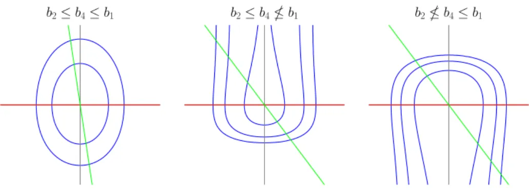
In the following figures, we illustrate our analysis of the ODE (3). Thereby, the red line is the u-nullcline, a₁u+b₁v =a₂u+b₂v, while the green line is the v-nullcline,a₃u+b₃v=a₄u+b₄v.

Figures 1, 2, 3, and 4 are illustrations of the proof of Lemma 5 on the bounded- ness of the solutions of the ODE (3). Figure 5 supports the proof of Theorem 7 on the characterization of global centers.

Figure 1: Phase portraits of the ODE (3) in case detJ > 0 and both of the diagonal entries ofJ are negative. As claimed in Lemma 4 (a), all solutions are bounded in positive time. Seven cases are ultimately monotonic, the remaining two (top left and bottom right) can spiral, but only inwards.

Figure 2: The forward invariant sets used in the proofs of Lemma 5 (b1) and (b2), respectively, to show the necessity of a₃≤a₂< a₁≤a₄ (top panel) and a₃ ≤a₂ =a₁ ≤a₄ (bottom panel) for the boundedness of the solutions of the ODE (3).

Figure 3: The level sets of the Lyapunov function used to show the sufficiency of a3 ≤a2 =a1 ≤a4 for the boundedness of the solutions of the ODE (3) in Lemma 5 (b2).

Figure 4: The bounded forward invariant sets used to show the sufficiency of a3 ≤ a2 = a1 ≤ a4 for the boundedness of the solutions of the ODE (3) in Lemma 5 (b2).