Linearizability problem of persistent centers

Linearizability problem of persistent centers

Matej Mencinger

, Brigita Ferˇcec

, Wilker Fernandes

and Regilene Oliveira

1University of Maribor, Faculty of Civil Engineering, Transportation Engineering and Architecture, Smetanova 17, 2000 Maribor, Slovenia

2Institute of Mathematics, Physics and Mechanics, Jadranska 19, 1000 Ljubljana, Slovenia

3Center for Applied Mathematics and Theoretical Physics, University of Maribor, Mladinska 3, 2000 Maribor, Slovenia

4University of Maribor, Faculty of Energy Technology, Hoˇcevarjev trg 1, 8270 Krško, Slovenia

5Departamento de Matemática e Estatística, Universidade Federal de São João del Rei, São João del Rei, Minas Gerais 36307-352, Brazil

6ICMC, Universidade de São Paulo, Avenida Trabalhador São-carlense, 400, 13566-590, São Carlos, SP, Brazil

Received 3 October 2017, appeared 4 June 2018 Communicated by Alberto Cabada

Abstract. The concepts of persistent and weakly persistent centers were introduced in 2009 and the same concept was applied in the study of some families of differential equations in 2013. Such concept was generalized for complex planar differential sys- tems in 2014. In this paper we extend the notion of persistent center to a linearizable persistent center and a linearizable weakly persistent center. Using the methods and al- gorithms of computational algebra we characterize the planar cubic differential system having linearizable persistent and linearizable weakly persistent centers at the origin.

Keywords: linearizability problem, center problem, focus quantities, persistent center.

2010 Mathematics Subject Classification: 34C25, 34M35, 37C10, 37C27.

1 Introduction

In the qualitative theory of differential systems there are many important open problems, for instance, the existence and number of limit cycles bifurcating from periodic orbits or singular points, problem of distinguishing between center and focus, linearizability problem, problem of critical periods etc. One of demanding problems is also characterizing centers and lineariz- able centers for a given planar polynomial differential system. A center of an analytic system is called a linearizable center if and only if there is an analytic change of coordinates which brings the original system to a linear system. To obtain conditions for linearizable centers one can compute the so called linearizability quantities whose vanishing ensures necessary and sufficient conditions for a center being linearizable (see Section 2 for more details). In spite

BCorresponding author. Email: brigita.fercec@um.si

of the capability of nowadays computers only the first few linearizability quantities can be computed. The problem also becomes more difficult with increasing of the number of param- eters of the considered system. Thus, linearizability problem as well as also center problem only for some special families of polynomial systems have been investigated (see for instance [2,3,7,9–15,18,27,28,30,31]).

In [4] the authors generalize the concept of a center by introducing the concept of persistent and weakly persistent centers for real differential systems. Such kind of problem is equivalent to find the systems with centers which are structurally stable under perturbations inside the same class of systems (i.e. polynomial systems, analytic systems, smooth systems, etc). The same concept also appears in [5] in the study of some Abel equations. In [3] the authors generalized the notion of persistent center and weakly persistent center to complex planar differential systems and found all conditions to get a persistent center in planar cubic systems and all conditions to get a weakly persistent center for complex cubic Lotka–Volterra system.

In this paper we introduce the concepts of linearizable persistent and linearizable weakly persistent centers and find necessary and sufficient conditions for planar cubic systems to have a linearizable persistent center. We also present the necessary and sufficient conditions for the existence of a linearizable weakly persistent center for the family of systems which define a kind of a generalization of the Kolmogorov systems.

2 Preliminaries

For planar analytic differential systems of the form

˙

u=−v+P(u,v), v˙ =u+Q(u,v), (2.1) where u,v ∈ _R and P,Q are analytic functions whose series expansions start from degree at least two, it is well-known that the origin can be either a focus or a center. The problem to distinguish between a center or a focus is called the center-focus problem. The origin O = (0, 0)is called a center of system (2.1) if it is surrounded by a family of periodic orbits.

By the Poincaré–Lyapunov theorem [20,25]Ois a center of (2.1) if and only if it admits a first integral of the form

Φ(u,v) =u²+v²+

∑

j+k≥3

φ_j,ku^jv^k.

One of the main difficulties in the study of the center problem comes from the complexity in computing the irreducible decomposition of the affine variety^*of the ideal generated by the Lyapunov quantities, which are the coefficients of the Poincaré first return map (see e.g. [29]).

Since it is easier to study complex varieties than real ones it is common to complexify the real system as follows. First settingx =u+ivfrom system (2.1) we obtain the equation

˙

x=ix+F(x,x), (2.2)

where i = √

−1, and F(x,x) = (P+iQ)((x+x)/2,(x−x)/2i). Adjoining to equation (2.2) its complex conjugate we get the system

˙

x=ix+F(x,x), x˙ =−ix+F(x,x).

*The affine variety of an ideal I = hf₁, . . . ,fsi ∈ k[x₁, . . . ,xn], where k is a field is the set V(I) = {a = (a1, . . . ,an)∈kⁿ: f_j(a) =0 for eachf_j∈I}.

Consider y := x as a new variable andG = F(x,x)as a new function we obtain a system of two complex differential equations which we write in the form

˙

x=ix+F(x,y), y˙ =−iy+G(x,y), (2.3) where x,y ∈ _C and F and G are analytic complex functions whose series expansions start from terms of degree at least two.

The next definition is natural in view of the Poincaré–Lyapunov theorem and the complex- ification procedure described above.

Definition 2.1 ([29]). System (2.3) has a complex center at the origin if it admits an analytic first integral of the form

Ψ(x,y) =xy+

∑

j+k≥3

ϕ_j,kx^jy^k. (2.4)

There are several generalizations of the classical center-focus problem. One of these no- tions is the following. The singular pointOin a complex systems of the form

˙

x= px+P(x,y), y˙= −qy+Q(x,y),

where x,y ∈_C, p,q∈ _{N, and}P,Q∈_C[x,y]is called a p:−qresonant center if there exists a local analytic first integral of the form

Φ(_x,y) =_x^q_y^p+

∑

j+k>p+q+1

φ_j−q,k−px^jy^k.

Some results for p:−qresonant centers can be found in [2,9,10,12,13,21,22,28,33]. A different approach to similar systems is presented in [26]. Some other generalizations are discussed also in [11] and [23]. The classical center-focus problem for a class of cubic systems was recently considered in [31].

Another generalization of the concept of center to real system was presented by [4].

Definition 2.2 ([4]). The origin of (2.2) is a persistent center (respectively, weakly persistent center) if it is a center for

˙

x= ix+λF(x,x), x∈_C for all λ∈ _C(respectively,λ∈_R).

Such concept was extended to the complex case by [3].

Definition 2.3 ([3]). The origin of (2.3) is a persistent center (respectively, weakly persistent center) if it is a center for

˙

x=ix+λF(x,y), y˙ =−iy+µG(x,y), x,y∈_C (2.5) for all λ,µ∈_C(respectively,λ=µ∈_C).

In [4] authors found some general systems of type (2.2) where the origin is a persistent center: a) ˙x =ix+Ax²+Cx²(quadratic), b) ˙x =ix+F(x), with F(0) = F⁰(0) =0 (holomor- phic), c) ˙x=ix+F(x), withF(0) =F⁰(0) =0 (Hamiltonian), d) ˙x=ix+xxF(x)(separated), and e) ˙x = ix+Bx^kx^lΨ(xx), with k 6= l+1 (reversible), where A,B,C ∈ _C andΨ a real an- alytic function such that the series expansion for x^kx^lΨ(xx) starts with second order terms.

Furthermore, for some special cases of (2.2), where

F(x,x) =Ax²+Bxx+Cx²+Dx³+Ex²x+Fxx²+Gx³,

the origin is proven to be a persistent center (see [4, Theorem 1.2]). This result was generalized in [3] to systems (2.3), see [3, Theorem 2.2].

If the singular point at the origin of system (2.1) is known to be a center we say that this center isisochronousif all periodic solutions of (2.1) in a neighbourhood of the origin have the same period. Moreover, system (2.1) is said to belinearizableif there is an analytic change of coordinates

u=u₁+Z(u₁,v₁), v=v₁+W(u₁,v₁), that reduces (2.1) to the canonical linear center

˙

u₁ =−v₁, v˙₁ =u₁.

Of course that there are similar definition for complex systems (2.3). The following theorem (see e.g. [29] for the details) shows us that there is an intimate relation between linearizability and isochronicity.

Theorem 2.4. Assume that the origin of (2.1) is a center. Then the origin is an isochronous center if and only if system(2.1)is linearizable.

It follows from Theorem2.4that solving the isochronicity problem is equivalent to solving the linearizability problem which is, from a computational point of view, much simpler.

Generalizing these concepts we introduce some new definitions concerning linearizability of persistent and weakly persistent centers of complex system (2.3).

Definition 2.5. The origin O is called an linearizable persistent center of system (2.3) if it is a persistent center and there exists an analytic change of coordinates of the form

x= x₁+

∑

j+k≥2

c_j,kx^j₁y^k₁, y=y₁+

∑

j+k≥2

d_j,kx₁^jy^k₁, that reduces (2.5) to the system

˙

x₁ =ix₁, y˙₁= −iy₁ (2.6)

for allλ,µ∈_C.

Definition 2.6. The originOis called alinearizable weakly persistent centerof system (2.3) if it is a weakly persistent center and system (2.5) is linearizable for allλ,µ∈_C.

The main goal of this paper is to study the linearizability of some planar cubic differen- tial systems. In Section3some computational techniques for the linearizability of persistent centers and wealky persistent centers are given. Applying these techniques and some other ideas, in Section4we present two main results. First, in Subsection4.1we give the necessary and sufficient conditions for the existence of an linearizable persistent center for the family of systems of the form

x˙ =ix+a20x²+a₁₁xy+a02y²+a30x³+a₂₁x²y+a₁₂y²x+a03y³,

˙

y= −iy+b₂₀x²+b₁₁xy+b₀₂y²+b₃₀x³+b₂₁x²y+b₁₂y²x+b₀₃y³, (2.7) and then, in Subsection4.2we present the necessary and sufficient conditions for the existence of an linearizable weakly persistent center for the family of systems which define a kind of a generalization of the Kolmogorov systems (which we call “semi-Kolmogorov” systems), i.e.

systems of the form

˙

x=ix+x a₂₀x+a₁₁y+a₃₀x²+a₂₁xy+a₁₂y² ,

˙

y= −iy+b₂₀x²+b₁₁xy+b₀₂y²+b₃₀x³+b₂₁x²y+b₁₂xy²+b₀₃y³. (2.8)

3 Linearizability of persistent centers

In this section a general approach used to study the classical linearizability problem and the linearizability problem for persistent centers and weakly persistent centers for complex sys- tems (2.3) is described. There are different algorithms to find the necessary conditions for lin- earizability (see e.g. [7,27,29]). Here we present a brief description of one of these algorithms.

The first step is the calculation of the linearizability quantities, denoted by i_k and j_k, which are polynomials in coefficients ofF(x,y)andG(x,y). For example, in case of (2.7) this means i_k,j_k ∈ _C[a,b], where a = (a₂₀,a₁₁,a₀₂,a₃₀,a₂₁,a₁₂,a₀₃) and b = (b₂₀,b₁₁,b₀₂,b₃₀,b₂₁,b₁₂,b₀₃). For any polynomial system (2.3) we use the parameters notation (a,b) in a similar way. We want to decide whether system (2.3) can be transformed into the linear system (2.6) by means of the inverse linearizing transformation

x₁= x+

∑

c_m−1,j(a,b)x^my^j, y₁=y+

∑

d_m−1,j(a,b)x^my^j. (3.1) If such a transformation exists, we say that the system is linearizable. Differentiation of each part of (3.1) with respect to t, applying (2.3) and (2.6), and then equating the coefficients of the termsx^q1+1y^q2 andx^q1y^q2+1yields the following recurrence formulae [29],

(q₁−q2)cq₁,q₁ =

q₁+q2−1 s1+

∑

(s₁+1)cs₁,s2aq₁−s₁,q2−s2−s2cs₁,s2bq₁−s₁,q2−s2

, (3.2)

(q₁−q₂)d_q1,q1 =

q1+q2−1 s₁+

∑

s₁d_s1,s2a_q1−s1,_q2−s2−(s₂+1)d_s1,s2b_q1−s1,_q2−s2

, (3.3)

where s₁,s₂ ≥ −1,q₁,q₂ ≥ −1, q₁+q₂ ≥ 0, c_1,−1 = c−1,1 = d_1,−1 = d−1,1 = 0, c_0,0 = d_0,0 =1, and we set a_p,q = b_p,q = 0 if p+q < 1. Using the recurrence formulae (3.2), (3.3) one can compute the coefficients c_q1,q2, d_q1,q2, whereq₁ 6= q₂. Forq₁ = q₂ = k the coefficientsc_k,k, d_k,k may be chosen arbitrary [29]. We setc_k,k =d_k,k =0. The system is linearizable if and only if all the polynomials forq₁ =q₂= k∈_Non the right hand side of (3.2), calledi_k, and on the right hand side of (3.3), called j_k, are equal to zero. The quantitiesi_k and j_k are calledlinearizability quantitiesfor polynomial system (2.3). This means that system (2.3) is linearizable if and only if

i_k(a,b) = j_k(a,b) =0, ∀k∈_N.

In the space of the parameters of a given polynomial family of systems (2.3) the set of all linearizable systems is the affine variety of the idealhi₁,j₁,i₂,j₂, . . .i, i.e. V(hi₁,j₁,i₂,j₂, . . .i).

Now, we restrict our attention to the cubic polynomial systems (2.7) and its respective family

x˙ = ix+λ a20x²+a₁₁xy+a02y²+a30x³+a₂₁x²y+a₁₂y²x+a03y³ ,

˙

y=−iy+µ b₂₀x²+b₁₁xy+b₀₂y²+b₃₀x³+b₂₁x²y+b₁₂y²x+b₀₃y³

. (3.4)

Obviously for any fixed λandµone can compute i_k = i_k(λ,µ,a,b) andj_k = j_k(λ,µ,a,b)for system (3.4) and obtain

i_k =

∑

m,n

i⁽_k^m,n)(a,b)λ^mµⁿ, j_k =

∑

m,n

j_k^(m,n)(a,b)λ^mµⁿ. (3.5)

We look at these linearizability quantities as polynomials inλ and µand denote the coeffi- cient ofλ^mµⁿ as i⁽_k^m,n) and j_k^(m,n) fori_k(λ,µ,a,b)and j_k(λ,µ,a,b), respectively, and call it the k_(m,n)−thpersistent linearizability quantity(according toi_k andj_k). If the origin is a linearizable center of (3.4) for all λ,µ ∈ C, then it is by Definition 2.5 a linearizable persistent center of (2.7).

Note, that by Theorem 2.1 of [3] one can always assume that λµ 6= 0 in (3.4). This gives rise to define the following sets of polynomials

L_k = ⁿi⁽_k^m,n), j⁽_k^m,n); m,n∈_N0, m+n6=0o

, k=1, 2, 3, . . . and the ideals

L^p:=hL₁,L₂, . . . ,L_k, . . .i, L_k^p:=hL₁,L₂, . . . ,L_ki.

According to Definition2.3 settingλ = µto (2.5) one can consider the linearizability of a possibly weakly persistent center. Now, one can consideri_k(λ,a,b)and j_k(λ,a,b)and define the coefficients, i⁽_k^m), j_k^(m), corresponding to λ^m in the series expansion of the linearizabilizy quantities

i_k =

∑

m

i⁽_k^m)(a,b)λ^m, j_k =

∑

m

j_k^(m)(a,b)λ^m, (3.6) and call them k_(m)−th weakly persistent linearizability quantities. Next, defining the following sets of polynomials

L^w_k =ⁿi⁽_k^m), j⁽_k^m); m∈_N^o, k =1, 2, 3, . . . one can define the ideals

L^wp:=hL^w₁,L^w₂, . . . ,L^w_k, . . .i, L^wp_k :=hL^w₁,L^w₂, . . . ,L^w_ki.

Note that the ideals L^wp, L^wp_k , L^p and L_k^p are ideals in the polynomial ring C[a,b]. By the Hilbert Basis Theorem (see e.g. [6]) any of them is finitely generated and every ascending chain of idealsL₁^p ⊂ L₂^p ⊂ L₃^p ⊂ · · · and L^wp₁ ⊂ L₂^wp ⊂ L^wp₃ ⊂ · · · stabilizes, which means that there exists N ≥ 1 such that for every k > N, L_k^p = L^p_N. Now one can define the corresponding persistent and weakly persistent linearizability variety for systems (2.5) in a natural way

VL^p =V(L^p), VL^wp =V(L^wp).

In the rest of the work we will search forV_L^p for systems (3.4) andV_L^wp for systems (3.4) with a02=_a03=0. Note that the persistent center variety and the persistent linearizability variety is much easier to obtain than the (regular) center variety and (regular) linearizability variety for a cubic system (2.7) since the corresponding persistent linearizability quantities, i⁽_k^m,n), j⁽_k^m,n), are split compared to (regular) linearizability quantitiesi_k(λ,µ,a,b)andj_k(λ,µ,a,b).

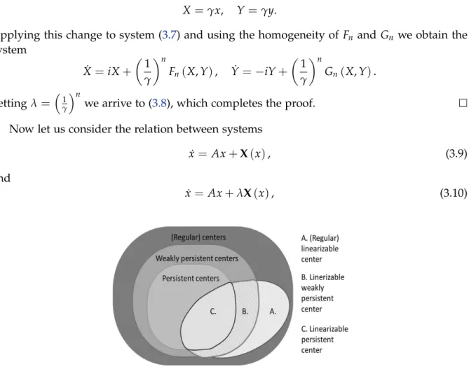
In Figure 3.1 the relation between the varieties of (regular) centers Vc, weakly persistent centersV_wpc, persistent centers V_pc, (regular) linearizable centersV_l, linearizable weakly per- sistent centers, and linearizable persistent centers for system (2.7) is presented.

In the next two propositions systems (2.3) and (2.5) are quasi-homogeneous systems of degree n, i.e. there exists n ≥ 2 such that F(tx,ty) = tⁿF(x,y) and G(tx,ty) = tⁿG(x,y),

∀x,y,t.

Proposition 3.1. If system(2.3)is quasi-homogeneous of degree n, n≥ 2, then the origin is a weakly persistent center if and only if it is a center.

See [3, pp. 114–115], for the proof.

Proposition 3.2. If system(2.3)is quasi-homogeneous of degree n, n≥2, then the origin is a lineariz- able weakly persistent center if and only if it is a linearizable center, i.e, VL^wp = VL,where VL^wp and V_Lare the weak persistent linearizability variety and the linearizability variety, respectively, of system (2.3).

Proof. Under the assumption of the proposition we write systems (2.3) and (2.5) forλ =µin the form

˙

x= ix+F_n(x,y), y˙ = −iy+G_n(x,y), (3.7) and

˙

x=ix+λF_n(x,y), y˙ = −iy+λG_n(x,y), (3.8) respectively, wheren≥2,Fn(x,y)andGn(x,y)are homogeneous polynomials of degreenin xandy.

We shall prove that system (3.7) is equivalent to system (3.8), up to a linear change of variables, so both systems must have the same linearizability varieties. In fact, for any γ6=0 consider the linear change of variables

X= γx, Y=γy.

Applying this change to system (3.7) and using the homogeneity ofF_n andG_n we obtain the system

X˙ =iX+ 1

γ n

Fn(X,Y), Y˙ =−iY+ 1

γ n

Gn(X,Y). Settingλ=¹

γ

n

we arrive to (3.8), which completes the proof.

Now let us consider the relation between systems

˙

x = Ax+X(x), (3.9)

and

˙

x= Ax+λX(x), (3.10)

Figure 3.1: The relation between the varieties Vc, Vpc, Vwpc and V_l, VL^p, VL^wp

VL^p ⊂VL^wp ⊂_C¹⁴ of the cubic system (2.7).

in terms of the linearizing transformation, where x ∈ _Cⁿ, λ ∈ _C, A is a complex matrix andX : C→_C is an analytic map starting with quadratic terms. Suppose that (3.9) can be linearized to

˙

y= Ay, (3.11)

by the linearizing transformation

x=y+_h(y).

Suppose that σ_A = {κ₁,κ₂, . . . ,κ_n}and A = diag(κ₁,κ₂, . . . ,κ_n)(i.e. A is in the Jordan form).

We follow the text in ([29, Sec. 2.2]) and denote

h(y) =h⁽²⁾(y) +h⁽³⁾(y) +· · ·+h^(k)(y) +· · · X(x) =X⁽²⁾(x) +X⁽³⁾(x) +· · ·+X^(k)(x) +· · ·

and write H_k for the linear space of all possible (vectorial) monomials. For example for x= (x₁,x2)∈_C² we have

H₂ =

x²₁ 0

,

x₁x₂ 0

,

x²₂ 0

,

0 x²₁

,

0 x₁x2

,

0 x²₂

. The basis elements ofH_k are usually written as x^α₁¹x^α₂², 0T

and 0,x^α₁¹x₂^α2T

. Denote κ= (κ₁,κ₂, . . . ,κ_n),

α= (α₁,α₂, . . . ,α_n). Now we define the homological operatorL:H_k → H_k as

L:p(y)7−→dp(y)Ay−Ap(y),

wheredpis the Jacobian matrix of p. In linear spaceH_k the eigenvalues, λ_k, of Lare defined by

λ_m =α·κ−κ_m.

Any monomialx^α₁¹x^α₂². . .x^α_nⁿ in the m-th component on the right hand side (RHS) of the sys- tems (3.9) and (3.10) for which α= (α₁,α₂, . . . ,α_n)satisfies the equation α·κ−κ_m =0 is said to beresonant.

Denote by K_k the complement to Image(L) in H_k. Note that resonant terms can not be removed from the normal form. They are elements ofK_k. Suppose thatK_k =∅^{for anyk} ≥2 for system (3.9). According to Theorem 2.2.3 of [29, Sec. 2.2] if for a system (3.9) for all k≥ 2 one hasK_k =∅, then this system can be linearized to (3.11).

In the following lemma we find the relation between the linearizing transformation of (3.10) and the linearizing transformation of (3.9). Byalet us denote all the parameters inX(x) from the RHS of (3.9) and (3.10). Note thath=h(a,y).

Lemma 3.3. Suppose thath=h(a,y)is a linearizing transformation of (3.9). Theneh=h(λa,y)is the linearizing transformation of (3.10).

Proof. Suppose that for allH_k,k≥2, the corresponding setK_k is empty for (3.9) and that dh^(k)(a,y)Ay−Ah^(k)(a,y) =X^(k)(y), (3.12) for ally, then

h(a,y) =h⁽²⁾(a,y) +h⁽³⁾(a,y) +· · ·+_h^(k)(a,y) +· · · _.

It is obvious that systems (3.9) and (3.10) have the same resonant terms. Therefore, there exist also the linearizing transformation for (3.10) which we denote byeh. ForheinH_k the setK_k is empty anddeh^(k)(y)Ay−Ahe^(k)(y) =λX^(k)(y)for ally.

Next we prove thatehcan be set to the formeh=h(λa,y). First note that for allk ≥ 2 and for all yandλ6=0 we have

h^(k)(λa,y) = ¹

λ^k−1h^(k)(a,λy) and X^(k)(y) = ¹

λ^kX^(k)(λy). (3.13) Substituting ybyλyin equation (3.12) and dividing it byλ^k−1 yields

1

λ^k−2dh^(k)(a,λy)· ¹

λAλy− ¹

λ^k−1Ah^(k)(a,λy) = ^λ

λ^kX^(k)(λy). Using equations (3.13) we rewrite the above equation in the form

dh^(k)(λa,y)Ay−Ah^(k)(λa,y) =λX^(k)(y),

which proves thath(λa,y)is a linearizing transformation for system (3.10).

Finally, we recall some notions about the Darboux linearizability and integrability theory which is the main tool for proving the sufficiency of the main Theorems 4.1 and 4.2 of this paper. For (2.3) the algebraic partial integral f and itscofactor k are polynomials defined by the equation

∂f

∂x (ix+F(x,y)) + ^∂f

∂y(−iy+G(x,y)) =k·f,

where the degree of the cofactor k is at most one less than the degree of system (2.3). We are looking for algebraic partial integrals f₀,f₁, . . . ,fs and g₀,g₁, . . . ,gt and their cofactors k₀,k₁, . . . ,k_sandl₁,l₂, . . . ,l_t and, in particular, for constantsα₁, . . . ,α_s,β₁, . . . ,β_t such that

k₀+α₁k₁+· · ·+α_sk_s= i, (3.14) and

l₀+β₁l₁+· · ·+βtlt= −i. (3.15) If such algebraic partial integrals, cofactors and constants are found, the linearizing transfor- mation (3.1) is of the form

x₁ = f₀f₁^α1· · · f_t^αt, y₁= g₀g^β₁¹· · ·g_t^βt. (3.16) Sometimes we can not find enough algebraic partial integrals to construct both Darboux lin- earizing transformations in (3.16). Let say that we can find only transformation x₁ which linearizes first equation of (2.3). In such case we can use first integral of (2.3). If we can find or at least prove the existence of first integral Ψof the form (2.4) then the second equation of system (2.3) can be linearized by transformation

y₁= ^Ψ

x₁ . (3.17)

In some cases the first integral can be also found (or be proven to exist) using the Darboux theory. If we can find a solution to the equation

∑

ψ_jK_j =0, (3.18)

whereK₁, . . . ,K_s are cofactors of some partial first integrals p₁, . . . ,p_sof system (2.3) then Ψ(x,y) = p^ψ₁¹p^ψ₂²· · ·p^ψ_s^s,

is the first integral of (2.3), which is called Darboux first integral.

If first integral Ψ(x,y) for (2.3) can not be found as described above, we can look for a differentiable function µ(x,y) defined on an open set Ω ⊆ _C², called an integrating factor.

In particular, for (2.3) the integrating factor is any solution (defined on Ω) to the following partial differential equation

∂µ(x,y)

∂x (ix+_F(_x,y)) +^∂µ(x,y)

∂y (−iy+_G(_x,y))

≡ −µ(x,y)

∂(ix+F(x,y))

∂x + ^∂(−iy+G(x,y))

∂y

.

If we have s algebraic partial first integrals p₁, . . . ,p_s with the corresponding cofactors K₁, . . . ,K_s and we are able to find constantsγ₁, . . . ,γ_ssuch that

∑

γ_jK_j+^∂(ix+F(x,y))

∂x + ^∂(−iy+G(x,y))

∂y ≡0, (3.19)

then

µ= p^γ₁¹· · ·p^γ_s^s,

is an integrating factor of (2.3), which is called the Darboux integrating factor. Using the obtained integrating factor we can then construct first integral of system (2.3). More details about Darboux integrability and linearizability an interesting reader can find in [29].

4 Main results

In this section we characterize the linearizable persistent center of type (2.7) and linearizable weakly persistent center of type (2.8)

4.1 Linearizable persistent centers of system (2.7)

Theorem 4.1. System (2.7)has a linearizable persistent center at the origin if and only if one of the following conditions holds:

(1) b₃₀ =b₂₁ =b₂₀=b₁₂= b₁₁= a₃₀ =a₂₁= a₂₀ =0, (2) b₃₀ =b₂₁ =b₂₀=b₁₂= b₁₁= a₃₀ =a₂₁= a₁₁ =0,

(3) b₃₀ =b₂₁ =b₂₀=b₁₂= b₁₁= a₂₁ =a₁₂= a₁₁ =a₀₃=a₀₂=0, (4) b₁₂ =b₁₁ =b03= a₂₁= a₁₂ =a₁₁= a03 =a02=0,

(5) b₁₂ =b₀₃ =b₀₂= a₂₁= a₁₂ =a₁₁= a₀₃ =a₀₂=0.

Proof. The linearizability quantities (3.5) of a complex cubic system (3.4) are polynomials in λ and µ with coefficients i⁽_k^m,n)(a,b), j⁽_k^m,n)(a,b) being polynomials in a and b. So (2.7) has a linearizable center at the origin for all λ,µ ∈ _C if and only if all polynomials i⁽_k^m,n)(a,b)_’s

and j_k^(m,n)(a,b)’s vanish (i.e. (a,b) ∈ VL^p). We compute the first seven pairs, i₁, j₁, . . . ,i₇, j₇, of linearizability quantities (3.5) of system (3.4). As the quantities are very large we present below only the first pair

i₁= a₂₁λ+ia₁₁a₂₀λ²−ia₁₁b₁₁λµ− ²

3ia₀₂b₂₀λµ, j₁= b₁₂µ+ia₁₁b₁₁λµ+²

3ia₀₂b₂₀λµ−ib₀₂b₁₁µ².

The next computational step is to compute the irreducible decomposition of the variety of ideal L^p = hL₁,L₂, . . .i. We use the routine minAssGTZ^** [8] of the computer algebra system SINGULAR [17]. Performing computations the same decomposition is obtained for V(L₅^p), V(L₆^p)andV(L₇^p), but forV(L₄^p)a different decomposition is obtained. This lead us to expect thatV(L^p) =_V(L₅^p)_.

The decomposition ofV(L₅^p)consists of five components listed in Theorem4.1 and these are necessary conditions for a linearizable persistent center at the origin of system (2.7).

Now we need to prove that each of these five conditions is also sufficient.

Case (1). Systems (2.7) and (3.4) are

˙

x=ix+a₁₁xy+a₀₂y²+a₁₂xy²+a₀₃y³, y˙ =−iy+b₀₂y²+b₀₃y³, (4.1) and

˙

x=ix+λ(a₁₁xy+a₀₂y²+a₁₂xy²+a₀₃y³), y˙ =−iy+µ(b₀₂y²+b₀₃y³), (4.2) respectively. System (4.2) has partial first integrals

g₀ =y, g₁ =1+ ¹

2i

µb₀₂−√ µ

q

4ib₀₃+µb²₀₂

y, g₂ =₁+ ¹

2i

µb₀₂+√ µ

q

4ib₀₃+µb²₀₂

y, with respective cofactors

l₀= −i+µb₀₂y+µb₀₃y², l₁= ¹

2

µb₀₂−√ µ

q

4ib₀₃+µb₀₂²

y+µb₀₃y², l₂= ¹

2

µb₀₂+√ µ

q

4ib₀₃+µb₀₂²

y+µb₀₃y². It is easy to verify that equation (3.15) is satisfied for

β₁=

√µb₀₂−^q4ib₀₃+µb²₀₂ 2

q

4ib₀₃+µb²₀₂

and β₂=−

√µb₀₂+ q

4ib₀₃+µb²₀₂ 2

q

4ib₀₃+µb₀₂² ,

so according to (3.16) we obtain that the second equation of (4.2) is linearizable by the change of coordinates

y₁ =yg₁^β1g^β₂².

**minAssGTZcomputes decomposition of the affine variety of the corresponding ideal into the irreducible com- ponents using the algorithm of [16].

In order to find a change of coordinates for the first equation of (4.2) we use (3.17). By Theorem 3.2 of [3], (4.2) possess a first integral Ψ(x,y). Thus, by (3.17), the first equation of (4.2) is linearizable by the change of coordinates x₁ = _Ψ/y1. Therefore, O is a linearizable persistent center of (4.1).

Case (2).Systems (2.7) and (3.4) are

˙

x=ix+a₂₀x²+a₀₂y²+a₁₂xy²+a₀₃y³, y˙ =−iy+b₀₂y²+b₀₃y³, (4.3) and

˙

x=ix+λ(a₂₀x²+a₀₂y²+a₁₂xy²+a₀₃y³), y˙ = −iy+µ(b₀₂y²+b₀₃y³), (4.4) respectively. System (4.4) has partial first integrals

g₀=y, g₁=1+¹

2i

µb02−√ µ

q

4ib03+µb²₀₂

y, g₂=1+¹

2i

µb₀₂+√ µ

q

4ib₀₃+µb²₀₂

y, with respective cofactors

l₀ = −i+µb₀₂y+µb₀₃y², l₁ = ¹

2

µb₀₂−√ µ

q

4ib₀₃+µb²₀₂

y+µb₀₃y², l2 = ¹

2

µb02+√ µ

q

4ib03+µb²₀₂

y+µb03y². It is easy to verify that equation (3.15) is satisfied for

β₁=

√µb02−^q4ib03+µb₀₂² 2

q

4ib₀₃+µb²₀₂

and β2= −

õb02+ q

4ib03+µb²₀₂ 2

q

4ib₀₃+µb²₀₂ ,

so according to (3.16) we obtain that the second equation of (4.2) is linearizable by the change of coordinates

y₁=yg^β₁¹g^β₂².

In order to find a change of coordinates for the first equation of (4.2) we use (3.17). By Theorem 3.2 (condition 7) of [3], (4.4) possess a first integralΨ(x,y). Thus, by (3.17), the first equation of (4.4) is linearizable by the change of coordinates x₁ = _Ψ/y1. Therefore, O is a linearizable persistent center of (4.3).

Case (3).Systems (2.7) and (3.4) are

˙

x =ix+a20x²+a30x³, y˙ =−iy+b02y²+b03y³, (4.5) and

˙

x=ix+λ(a₂₀x²+a₃₀x³)_, y˙ =−iy+µ(b₀₂y²+b₀₃y³)_{, (4.6)}

respectively. System (4.6) has partial first integrals l₁ =x,

l₂ =1− ¹ 2i

λa₂₀−√ λ

q

−4ia₃₀+λa²₂₀

x, l₃ =1− ¹

2i

λa₂₀+√ λ

q

−4ia₃₀+λa²₂₀

x, l₄ =y,

l5 =1+ ¹ 2i

µb02−√ µ

q

4ib03+µb²₀₂

y, l₆ =1+ ¹

2i

µb₀₂+√ µ

q

4ib₀₃+µb²₀₂

y, with respective cofactors

k₁ =i+λa₂₀x+λa₃₀x², k₂ = ¹

2

λa₂₀−√ λ

q

−4ia₃₀+λa²₂₀

x+λa₃₀x², k₃ = ¹

2

λa₂₀+√ λ

q

−4ia₃₀+λa²₂₀

x+λa₃₀x², k₄ = −i+µb02y+µb03y²,

k5 = ¹ 2

µb02−√ µ

q

4ib03+µb²₀₂

y+µb03y², k₆ = ¹

2

µb₀₂+√ µ

q

4ib₀₃+µb²₀₂

y+µb₀₃y².

It is easy to verify that choosing f₀= l₁, f₁ =l₂and f₂ =l₃equation (3.14) is satisfied for

α₁=

√λa₂₀−^q−4ia₃₀+λa²₂₀ 2

q

−4ia₃₀+λa²₂₀

and α₂=−

√λa₂₀+ q

−4ia₃₀+λa²₂₀ 2

q

−4ia₃₀+λa²₂₀ ,

and choosing g0 =l₄, g₁= l5 andg2 =l6, equation (3.15) is satisfied for

β₁=

√µb02−^q4ib03+µb²₀₂ 2

q

4ib₀₃+µb²₀₂

and β₂=−

õb02+ q

4ib03+µb²₀₂ 2

q

4ib₀₃+µb₀₂² .

So we obtain that (4.6) is linearizable by the change of coordinates x₁= x f₁^α1f₂^α2, y₁=yg₁^β1g^β₂². Therefore,Ois a linearizable persistent center of (4.5).

Case (4). System (2.7) satisfying conditions (4) of this theorem can be transformed into system (4.3), where

(a20,a30,b02,b20,b₂₁,b30) =−(b02,b03,a20,a02,a₁₂,a03),

by the change of coordinates (x,y,t) → (y,x,−t). Therefore, O is a linearizable persistent center for this case.

Case (5). System (2.7) satisfying conditions (5) of this theorem can be transformed into system (4.1), where

(a₂₀,a₃₀,b₁₁,b₂₀,b₂₁,b₃₀) =−(b₀₂,b₀₃,a₁₁,a₀₂,a₁₂,a₀₃),

by the change of coordinates (x,y,t) → (y,x,−t). Therefore, O is a linearizable persistent center for this case.

4.2 Linearizable weakly persistent centers of system (2.8)

In order to perform the complete analysis of linearizbility problem for a weakly persistent center of system (2.7) even using powerful computer we were not able to carry out compu- tations of decomposition of varietyV(I), where I is an ideal generated by first seven pairs of linearizability quantities. We also tried to obtain decomposition over the finite field of characteristics 32003 but computations were again too laborious. Therefore, we restrict our attention to systems (2.7) with a₀₃ = 0 and a₀₂ = 0, i.e. system (2.8), which is also called semi-Kolmogorov system. Kolmogorov systems are an important class of systems due to its wide use in mathematical biology to describe the interaction of two populations. In fact Kol- mogorov systems are a general model for the dynamics of biological species because it is the simplest model to describe the interaction of two species occupying the same ecological niche, see [19]. In that sense, they are generalizations of the so-called Lotka–Volterra systems, see [24,32]. We see that system (2.8) is larger family than Kolmogorov systems and it is the largest family for which we were able to find decomposition of varietyV(I).

Note that the Lotka–Volterra systems considered in [3], [7] and [27] are all subcases of (2.8) for which we state the following result.

Theorem 4.2. System(2.8) has a linearizable weakly persistent center at the origin if and only if one of the following conditions holds

(1) b₂₁ =b₂₀ =b₁₂=b₁₁= b₀₃= a₃₀ =a₂₁= a₂₀ =a₁₂=b₀₂−3a₁₁=0, (2) b₃₀ =b₂₁ =b₁₂=b₁₁= b₀₂= a₃₀ =a₂₁= a₂₀ =a₁₁=2a₁₂−b₀₃=_0, (3) b₃₀ =b₂₁ =b₂₀=b₁₂= b₁₁= a₃₀ =a₂₁= a₂₀ =0,

(4) b₂₁ =b₂₀ =b₁₂=b₁₁= a₃₀ =a₂₁= a₂₀=3a₁₂−b₀₃=3a₁₁+b₀₂=0, (5) b₃₀ =b₂₁ =b₂₀=b₁₂= b₁₁= a₃₀ =a₂₁= a₁₁ =0,

(6) b₃₀ =b₂₁ =b₂₀=b₁₂= b₁₁= a₂₁ =a₂₀= a_a12=2a₁₁+b₀₂=0, (7) b₃₀ =b₂₁ =b₂₀=b₁₂= b₁₁= a₂₁ =a₁₂= a₁₁ =0,

(8) b₃₀ =b₂₁ =b₂₀=b₁₂= b₀₂= a₃₀ =a₂₁= a₁₁ =a₂₀−2b₁₁ =a₁₂−2b₀₃ =0, (9) b₃₀ =b₂₁ =b₂₀=b₁₂= b₀₂= a₂₁ =a₁₂= a₁₁ =a₂₀+2b₁₁ =0,

(10) b₃₀ =b₁₂ =b₁₁=b₀₃= a₂₁ =a₂₀= a₁₂=2a₃₀−b₂₁=2a₁₁−b₀₂=0, (11) b₁₂ =b₁₁ =b₀₃= a₂₁= a₁₂ =a₁₁=0,

(12) b₃₀ =b₁₂ =b₁₁= a₂₁= a₁₁ =a₃₀−b₂₁ =a₁₂−b₀₃ =0, (13) b₁₂ =b₀₃ =b₀₂= a₂₁= a₁₂ =a₁₁=0,

(14) b₃₀ =b₂₀ =b₁₂= a₂₁= a₃₀−b₂₁= a₂₀−b₁₁ =a₁₂−b₀₃ =a₁₁−b₀₂=b₀₃b₁₁² +b²₀₂b₂₁ =_0.