Existence of a homoclinic orbit in a generalized Liénard type system

Existence of a homoclinic orbit in a generalized Liénard type system

Tohid Kasbi Gharahasanlou

, Vahid Roomi

and Aliasghar Jodayree Akbarfam

1Faculty of Mathematics, University of Tabriz, Tabriz, Iran

2Department of Mathematics, Azarbaijan Shahid Madani University, Tabriz, Iran

Received 24 August 2020, appeared 14 April 2021 Communicated by Gabriele Villari

Abstract. The object of this paper is to study the existence and nonexistence of an im- portant orbit in a generalized Liénard type system. This trajectory is doubly asymptotic to an equilibrium solution, i.e., an orbit which lies in the intersection of the stable and unstable manifolds of a critical point. Such an orbit is called a homoclinic orbit.

Keywords: Liénard system, homoclinic orbit, planar system, dynamical systems 2020 Mathematics Subject Classification: 34C37, 34A12, 34C10.

1 Introduction

Consider the planar system

˙

x= P(Q(y)−F(x))

˙

y=−g(x), (1.1)

which is a generalized Liénard type system, where P, Q, F and g are continuous functions satisfying suitable assumptions in order to ensure the existence of a unique solution to the initial value problems. Moreover, suppose that the following assumptions hold under which the origin is the unique critical point of system (1.1).

P(u)andQ(y)are strictly increasing andF(0) =P(0) =Q(0) =0, uP(u)>0 foru6=0,yQ(y)>0 fory6=0 andxg(x)>0 forx6=0.

System (1.1) includes the classical Liénard system as a special case, which is of great impor- tance in various applications (see [1] to [23] and the references cited therein).

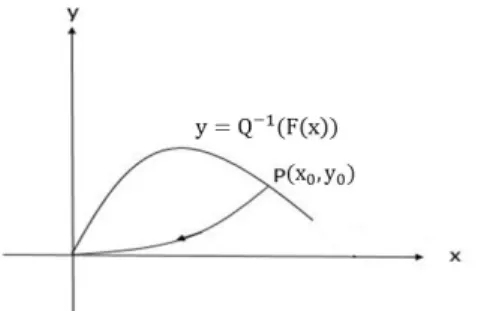
Definition 1.1. In system (1.1), a trajectory is said to be a homoclinic orbit if itsα- andω-limit sets are the origin (see Fig.1.1).

BCorresponding author. Email: roomi@azaruniv.ac.ir

Figure 1.1: Homoclinic orbit

The main purpose of this paper is to give an implicit necessary and sufficient condition and some explicit sufficient conditions onF(x),g(x),P(u)andQ(y) under which system (1.1) has homoclinic orbits. These results extend and improve the results presented for special cases of system (1.1) in [3,11,19].

The existence of homoclinic orbit is an important problem in nonlinear dynamical systems and the theory of ordinary differential equations. The results about the existence of homoclinic orbits for the other systems, such as the Lorenz system, Schrödinger systems, predator–prey systems and Hamiltonian systems can be found in [13,18,22,23], respectively. Moreover, vari- ous systems and equations such as generalized Euler equation [4] and predator–prey systems [22] can be transformed to the Liénard type systems.

The existence of homoclinic orbits in the Liénard-type systems is closely connected with the stability of the zero solution and the center problem (see [6,11,19,21]). If system (1.1) has a homoclinic orbit, then the zero solution is no longer stable. A homoclinic orbit and a center cannot exist together in system (1.1). Our subject also has a near relation with the global attractivity of the origin and oscillation of solutions and so on (see [9,12,20]).

The curveΓ= {(x,y)|y= Q⁻¹(F(x))}is called the characteristic curve of (1.1). Let Γ1={(x,y)|y=Q⁻¹(F(x))andx>0},

and

Γ2={(x,y)|y=Q⁻¹(F(x))_andx<₀}_.

Then, Γ = _Γ1^S_Γ2^S(0, 0). Positive and negative orbits of (1.1) passing through p ∈ _R² are shown by O⁺(p)and O⁻(p), respectively.

The following definitions are presented to state our main results.

Definition 1.2. System (1.1) has property(Z⁺₁)(resp.,(Z⁺₃)) if there exists a point p(x₀,y₀)∈ Γ1 (resp., p(x₀,y₀) ∈ _Γ2), such that the O⁺(p) of (1.1) starting at p approaches the origin through only the first (resp., third) quadrant (see Fig. 1.2).

Definition 1.3. System (1.1) has property(Z⁻₂)(resp.,(Z⁻₄)) if there exists a point p(x₀,y₀)∈ Γ2 (resp., p(x0,y0) ∈ _Γ1), such that the O⁻(p) of (1.1) starting at p approaches the origin through only the second (resp., fourth) quadrant.

If system (1.1) has both properties (Z₁⁺) and (Z₂⁻), then a homoclinic orbit exists in the upper half-plane. Similarly, if system (1.1) has both properties(Z⁺₃)_and(Z₄⁻), then a homo- clinic orbit exists in the lower half-plane. In this paper we will find conditions for deciding whether system (1.1) has homoclinic orbit.

Hara and Yoneyama in [9] considered system (1.1) with Q(y) = y and P(u) = u and presented some sufficient conditions under which the system has or fails to have property (Z₁⁺). Also, Sugie presented an implicit necessary and sufficient condition for system (1.1) with P(u) =u to have property (Z⁺₁)[19]. Next, Aghajani and Moradifam in [3] considered

Figure 1.2: Property(Z⁺₁)

system (1.1) with P(u) = u and gave an implicit necessary and sufficient condition for the system to have property (Z⁺₁)which improved some results in [19].

In the next section an implicit necessary and sufficient condition and some explicit suffi- cient conditions are provided for system (1.1) to have property(Z₁⁺). Since some nonlinear functions are added to the classical Liénard system in this article, our results are proper ex- tensions of the known ones in [3], [9], [11] and [19].

2 Necessary and sufficient conditions for property of ( Z

)

In this section we will give necessary and sufficient conditions for system (1.1) to have prop- erties (Z₁⁺) and (Z₂⁻). First, consider the following lemma about asymptotic behavior of solutions of (1.1).

Lemma 2.1. For each point H(c,Q⁻¹(F(c)))with c>0or c<0, the positive or negative semi-orbit of (1.1)starting at H crosses the negative y-axis if the following condition holds.

(A1) There exists a δ > 0 such that F(x) < 0for −δ < x < δ or F(x) has an infinite number of positive zeroes clustering at x=0.

Remark 2.2. Lemma 2.1 implies that system (1.1) fails to have properties (Z₁⁺) and (Z₂⁻) if (A1) holds. Hence, hereafter we assume that there exists a δ > 0 such that F(x) > _{0 for}

−δ <x< δ.

Theorem 2.3. System (1.1) has property (Z⁺₁) if and only if there exist a constant δ > 0 and a continuous functionφ(x)such that

0≤φ(x)< F(x) and Z _x

0

−g(η)

P(φ(η)−F(η))^dη≤ Q⁻¹(φ(x)) (2.1) for0<x <δ.

Proof. First, note that the positive semi-orbit of (1.1) starting at H(x₀,Q⁻¹(F(x₀)))is consid- ered as a solutiony(x)of

dy

dx = −g(x)

P(Q(y)−F(x))^{, (2.2)}

with y(x₀) =Q⁻¹(F(x₀))_.

Sufficiency: Suppose that system (1.1) fails to have property(Z₁⁺). Thus, there exist a point H(x0,Q⁻¹(F(x0)))andx0 >0 such that the positive semi-orbit of (1.1) starting at Hdoes not approach the origin through the first quadrant. Taking the vector field of (1.1) into account, it is obvious that the positive semi-orbit rotates in clockwise direction about the origin. For this reason, it crosses the curvey= Q⁻¹(φ(x))and meets the y-axis at a point(0,y₁)with y₁ <0.

Let

x₁=inf{x : 0<x< δ and y(x)> Q⁻¹(φ(x))}.

Then, (_x1,y(_x1)) is the intersection point of O⁺(_H) and the curvey = _Q⁻¹(φ(_x))_{nearest to} the origin, that isy(x₁) = Q⁻¹(φ(x₁))andy < Q⁻¹(φ(x))for 0 < x < x₁. Hence, from (2.1), it can be concluded that

Q⁻¹(φ(x₁))<y(x₁)−y₁ =

Z _x

0

−g(η)

P(Q(y(η))−F(η))^dη

<

Z _x1

0

−g(η)

P(φ(η)−F(η))^dη≤Q⁻¹(φ(x₁)), which is a contradiction.

Necessity: Suppose that O⁺(H) approaches the origin through the first quadrant. Then, its corresponding solutiony(x)satisfies

y(x)→0⁺ asx→0. (2.3)

Letδ= x₀ andφ(x) =Q(y(x))_{for 0}< x<δ. It is obvious thatφ(x)≥_{0. Thus,} Q⁻¹(φ(x)) =y(x)< Q⁻¹(F(x)),

and therefore,φ(x)< F(x)for 0<x <δ. Also, from (2.3) it can be easily seen that Z _x

0

−g(η)

P(φ(η)−F(η))^dη=

Z _x

0

−g(η)

P(Q(y(η))−F(η))^dη=y(x)−lim

e→0y(e)

=Q⁻¹(φ(x)). Thus, (2.1) holds and the proof is complete.

Remark 2.4. For P(u) =u, Theorem2.3gives the corresponding result of Sugie in [19].

Corollary 2.5. Suppose that there exists k∈(0, 1)andδ >0such that 1

Q⁻¹(kF(x))

Z _x

0

−g(η)

P((k−1)F(η))^dη≤1 for0<x< δ. (2.4) Then, system(1.1)has property(Z₁⁺).

Proof. Letφ(_x) =_kF(_x). The following inequality is obtained from (2.4).

Z _x

0

−g(η)

P(φ(η)−F(η))^dη=

Z _x

0

−g(η)

P((k−1)F(η))^dη≤Q⁻¹(kF(x)), for 0< x<δ. Thus, by Theorem2.3system (1.1) has property(Z₁⁺)_.

Corollary 2.6. Suppose that P(au)≤ aP(u)for a∈(−1, 0)and u >0. If there exist k∈(0, 1)and δ>0such that

1

(1−k)Q⁻¹(kF(x))

Z _x

0

g(η)

P(F(η))^dη≤1 for0< x<δ, then system(1.1)has property(Z₁⁺).

Remark 2.7. For P(u) = u and Q(y) = y and taking k = ¹₂, Corollary 2.6 gives the result of Hara and Yoneyama in [9].

Corollary 2.8. If for every k∈ [0, 1]there exists a constantγ_k >0such that lim inf

x→0⁺

1

Q⁻¹((k+γ_k)F(x))

Z _x

0

−g(η)

P((k−γ_k−1)F(η))^dη

>1, (2.5) then system(1.1)fails to have property(Z₁⁺).

Proof. Suppose that there exist a constantδ >0 and a continuous functionφsuch that condi- tion (2.1) holds. Definek⁰ =lim inf_x→0^{+ φ}_F⁽₍^x_x⁾₎. Then 0≤k⁰ ≤ 1, and from the definition ofk⁰ it follows that for every e> 0, there exist aband asequence {xn}with 0< b< δ, 0< xn ≤ b, andx_n→0 asn→+_∞such that

φ(x)

F(x) >k⁰−e for 0<x ≤b and φ(xn)

F(x_n) <k⁰+e.

Hence,

φ(x)>(k⁰−e)F(x) for 0< x≤b and φ(x_n)<(k⁰+e)F(x_n). Thus, from (2.1) it can be concluded that

0≥

Z _xn

0

−g(η)

P(φ(η)−F(η))^dη−Q⁻¹(φ(xn))

>

Z _xn

0

−g(η)

P((k⁰−e)F(η)−F(η))^dη−Q⁻¹((k⁰+e)F(x_n))_. Consequently, for n≥1 the following inequality holds.

1

Q⁻¹((k⁰+e)F(x_n))

Z _xn

0

−g(η)

P((k⁰−e−1)F(η))^dη<1. (2.6) Thus, (2.6) contradicts (2.5) and the proof is complete.

Corollary 2.9. Suppose that P(au)≥ aP(u)for a ∈ [−2,−1)and u > 0. If there exists β∈ (1, 2] such that

lim inf

x→0⁺

1

2Q⁻¹((β+1)F(x))

Z _x

0

g(η) P(F(η))^dη

>1, (2.7)

then system(1.1)fails to have property(Z₁⁺).

Proof. Suppose that (2.7) holds. Then, in (2.5) for every k ∈ [0, 1] let γ_k = (β−1)k+1. By this argument, we have k−1−γ_k = 2k−βk−2 and k+γ_k = βk+1. Since 1 < β ≤ 2 and 0≤k ≤_{1, then}

−2≤2k−βk−2< −1, 1

2 ≤ ¹

2+ (β−2)k <1 and βk+1≤β+1.

Now, put the last relations in the left-hand side of (2.5) and get lim inf

x→0⁺

1

Q⁻¹((k+γ_k)F(x))

Z _x

0

−g(η)

P((k−γ_k−1)F(η))^dη

=lim inf

x→0⁺

1

Q⁻¹((βk+1)F(x))

Z _x

0

−g(η)

P((2k−βk−2)F(η))^dη

≥_{lim inf}

x→0⁺

1

(2+ (β−2)k)Q⁻¹((β+1)F(x))

Z _x

0

g(η) P(F(η))^dη

≥_{lim inf}

x→0⁺

1

2Q⁻¹((β+1)F(x))

Z _x

0

g(η) P(F(η))^dη

>_1.

This completes the proof.

By choosing k = 0 in the proof of Corollary 2.9, the following corollary can be presented with weaker conditions.

Corollary 2.10. Suppose that P(au)≥aP(u)for a∈[−2,−1)and u >0. If lim inf

x→0⁺

1 2Q⁻¹(F(x))

Z _x

0

g(η) P(F(η))^dη

>1, (2.8)

then system(1.1)fails to have property(Z⁺₁).

The following corollaries can be obtained as results of Theorem2.3 which are very useful in applications.

Corollary 2.11. Suppose that system(1.1)with P(u) =P₁(u)has (resp., fails to have) property(Z⁺₁). If P2(u)≤ P₁(u)(resp., P2(u)≥ P₁(u)) for u <0, then system(1.1)with P(u) = P2(u)has (resp., fails to have) property(Z₁⁺).

Corollary 2.12. Suppose that system (1.1) with Q(y) = Q₁(y) has (resp., fails to have) property (Z₁⁺). If Q₂(y)≤ Q₁(y)(resp., Q₂(y)≥ Q₁(y)) for y>₀sufficiently small, then system(1.1)with Q(y) =Q₂(y)has (resp., fails to have) property(Z₁⁺).

By the same way, we can prove the following theorem about property(Z₂⁻).

Theorem 2.13. System (1.1) has property (Z₂⁻) if and only if there exist a constant δ > 0 and a continuous functionφ(x)such that

0≤ φ(x)< F(x) and Z _x

0

−g(η)

P(φ(η)−F(η))^dη≤Q⁻¹(φ(x)) for−δ <x<0.

Similarly, other obtained results (Corollaries2.5–2.10) can be formulated for property(Z⁻₂).

3 Some explicit results

Condition (2.1) is implicit necessary and sufficient for system (1.1) to possess property (Z⁺₁). However, in some cases, it is very difficult to find a suitable function φ(x)with a constantδ satisfying (2.1). Therefore, in the following, some explicit sufficient conditions are provided

for system (1.1) to have property (Z⁺₁). The results can also be formulated for the property (Z₃⁺),(Z₂⁻)or(Z₄⁻). We leave the details to the reader. To state the results, define

H(y) =

Z _y

0 Q(η)dη and G(x) =

Z _x

0 g(η)dη.

Also, the inverse function ofω(y) =H(y)sgn(y)is denoted by H⁻¹(ω).

Theorem 3.1. Suppose that P(au) ≤ aP(u)for a ∈ (−1, 0) and u > 0 and there existα > 0 and k∈[0, 1)such that

Q x

α(1−k)

≤kP⁻¹(αQ(x)) _(3.1)

for x >0sufficiently small. Then, system(1.1)has property(Z₁⁺)if

F(x)≥ P⁻¹(αQ(H⁻¹(G(x)))), (3.2) for x >0sufficiently small.

Proof. From (3.1) it is obvious that

u

α(1−k)Q⁻¹(kP⁻¹(αQ(u))) ≤1, (3.3) foru>0 sufficiently small. Since the functionu(x) =H⁻¹(G(x))is increasing and continuous on [0,∞)andu(0) =0, by (3.2) we obtain

H⁻¹(G(x))

α(1−k)Q⁻¹(kP⁻¹(αQ(H⁻¹(G(x))))) ≤1, (3.4) forx >0 sufficiently small. Since

d

dxH⁻¹(G(x)) = ^g(x) Q(H⁻¹(G(x)))^, from (3.4) we conclude that

1

(1−k)Q⁻¹(kF(x))

Z _x

0

g(η) P(F(η))^dη

≤ ¹

(1−k)Q⁻¹(kP⁻¹(αQ(H⁻¹(G(x)))))

Z _x

0

g(η)

αQ(H⁻¹(G(η)))^dη

= ^H

−1(G(x))

α(₁−k)Q⁻¹(kP⁻¹(αQ(H⁻¹(G(x))))) ≤1,

forx >0 sufficiently small. Hence, by Corollary2.6 system (1.1) has property(Z₁⁺).

By choosing α = 2, k = ¹₂ and P(u) = u, condition (3.1) holds for any function Q. In this case, the following corollary is obtained about property(Z₁⁺)which is the corresponding result of Sugie in [19].

Corollary 3.2. Suppose that

F(x)≥2Q(H⁻¹(G(x))), (3.5) for x >₀sufficiently small. Then, system(1.1)with P(u) =u has property(Z⁺₁).

Theorem 3.3. Suppose thatα > 0and P(au) ≥ aP(u)for a ∈ [−2,−1)and u > 0. Also, assume that there existsβ∈(1, 2]such that

Q x

2α

≥(β+1)P⁻¹(αQ(x)) (3.6) for x>₀sufficiently small. Then, system(1.1)fails to have property(_Z⁺₁)_if

F(x)≤ P⁻¹(λαQ(H⁻¹(G(x)))), (3.7) for someλ<1.

Proof. By (3.6) it is obvious that

u

αQ⁻¹((β+1)P⁻¹(αQ(u))) ≥2.

By the similar argument to the proof of Theorem3.1, it can be concluded that if (3.6) and (3.7) hold, then

lim inf

x→0⁺

1

2Q⁻¹((β+₁)F(x))

Z _x

0

g(η) P(F(η))^dη

>1.

Hence, by Corollary2.9system (1.1) fails to have property(Z₁⁺).

4 Homoclinic orbit

In this section some results will be presented about the existence of homoclinic orbit in the upper half-plane for system (1.1). The following theorem is obtained by combining Theorem 2.3and2.13.

Theorem 4.1. System (1.1) has homoclinic orbit in the upper half-plane if and only if there exist a constantδ>0and a continuous functionφ(x)such that

0≤ φ(x)< F(x) and Z _x

0

−g(η)

P(φ(η)−F(η))^dη≤Q⁻¹(φ(x)) (4.1) for0<|x|< δ.

The following two corollaries are obtained from Theorem4.1, which provide explicit con- ditions for system (1.1) to have homoclinic orbit in upper half-plane. Note that, in Remark2.2, it is assumed that there exists aδ>0 such thatF(x)>0 for−δ <x< δ.

Corollary 4.2. Suppose that there exist k∈(0, 1)andδ>0such that 1

Q⁻¹(kF(x))

Z _x

0

−g(η)

P((k−1)F(η))^dη≤1 for0< |x|< δ. (4.2) Then, system(1.1)has homoclinic orbit in the upper half-plane.

Corollary 4.3. Suppose that P(au)≤ aP(u)for a∈(−1, 0)and u>0. If there exist k∈ (0, 1)and δ>₀such that

1

(1−k)Q⁻¹(kF(x))

Z _x

0

g(η)

P(F(η))^dη≤1 for0< |x|< _{δ, (4.3)} then system(1.1)has homoclinic orbit in the upper half-plane.

Remark 4.4. Suppose that F is an even andgis an odd function. It is easy to see that system (1.1) has property (Z₁⁺) if and only if it has property (Z⁻₂). Therefore, if system (1.1) has property(Z₁⁺), then it has a homoclinic orbit in the upper half-plane.

Similarly, Theorem3.1 and Corollary3.2 and some other results can be formulated about property (Z₂⁻) and the existence of homoclinic orbits in the upper half-plane. Turning our attention to the lower half-plane, all presented results can be formulated about properties (Z₃⁺)and(Z₄⁻)and finally about the existence of homoclinic orbit in the lower half-plane.

In the following, two examples will be presented to illustrate our results and show the applications of the results.

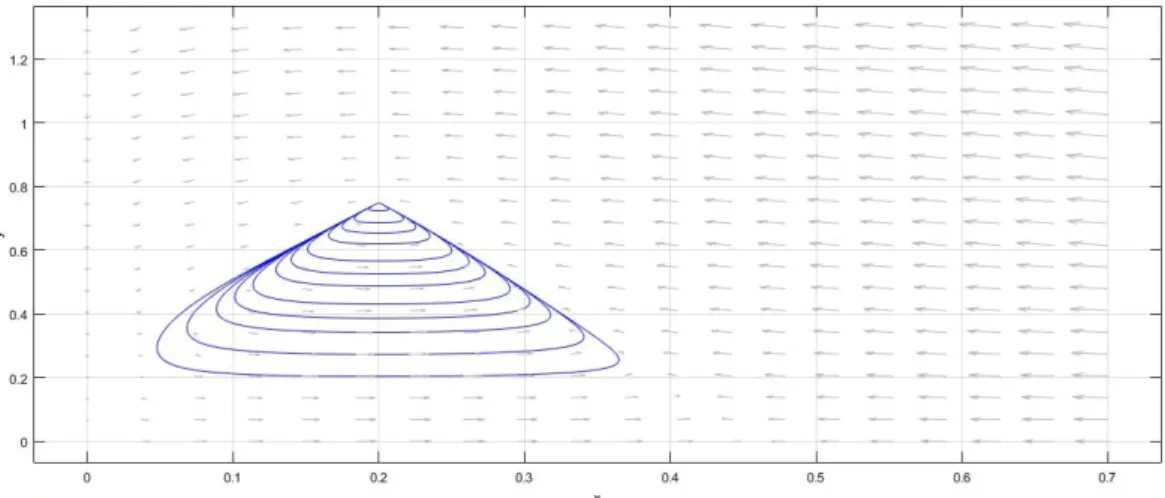
Example 4.5. Consider the following Gause-type Predator-Prey system u˙ =ur(u)−vs f(u)

˙

v =v(q(u)−D)_, ^(4.4)

with f(u) = u, r(u) = β−γ|u−α|, q(u) = u², D = α² and β > αγ. In system (4.4), u(t) andv(t)represent prey and predator densities, the function f(u)is functional response,q(u) is the growth rate of the predator, r(u) is the growth rate of the prey in the absence of any predators, and D > 0 is the natural death rate of the predator in the absence of any prey.

The constants α, β and γ are positive ecological parameters. System (4.4) has the positive equilibriumE^∗= (α,β). By the change of variables

x=u−α, y =lnβ−lnv and dt=uds, system (4.4) will be transformed into system (1.1) with

P(u) =u, Q(y) =β(1−e^−y), F(x) =γ|x| and g(x) =x+α− ^α

2

x+α. (4.5) Functions F(x) and g(x) are defined on (−α,+_∞) and satisfy F(0) = 0 and xg(x) > 0 for x 6= 0. Also,Q(y)is defined onR satisfyingQ(0) =0 and yQ(y)> 0 fory 6= 0. The inverse function of Q(y) isQ⁻¹(y) =ln _β−^β_y

where defined on(−_∞,β). For 0 < x < _kγ^β , by using Corollary4.3, it can be written that

1

(1−k)Q⁻¹(kF(x))

Z _x

0

g(η)

P(F(η))^dη= ¹ γ(1−k)ln

β β−kγx

x+αln

1+ ^x α

< ^2β

γ²(₁−k)k. By choosingk= ¹₂, it can be concluded that

1

(1−k)Q⁻¹(kF(x))

Z _x

0

g(η)

P(F(η))^dη< ^8β γ². If 0<_8β≤γ², then

1

(1−k)Q⁻¹(kF(x))

Z _x

0

g(η)

P(F(η))^dη<1.

By a similar argument, it can be shown that for −α<x <0 1

(1−k)Q⁻¹(kF(x))

Z _x

0

g(η)

P(F(η))^dη<1.

Figure 4.1: Phase portrait for system (4.4) with α=0.2,β=0.75 andγ=3.

Therefore, by Corollary 4.3 this system has a homoclinic orbit in the upper half-plane (see Fig.4.1).

Remark 4.6. Sugie and Kimoto in [22], under the assumption Q(y) ≤ my fory > 0, showed that system (1.1) with functions in (4.5) has homoclinic orbits in the upper half-plane if 0 <

8β ≤ γ². In this work, the existence of homoclinic orbits has been presented without the assumptionQ(y)≤myfory>0.

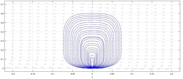
Example 4.7. Consider system (1.1) with functions P(u) =u³, Q(y) =sgn(y)

q

|y|, F(x) = ⁴ q

|x| and g(x) =x. (4.6) By Corollary2.5, it can be written that

1 Q⁻¹(kF(x))

Z _x

0

−g(η)

P((k−1)F(η))^dη= ⁴

√4

x³

5k²(1−k)³ ≤1 for 0 < x < ³₅^{4 1}

5√³

5. Therefore, this system has property (Z₁⁺). Since F is even and g is odd, Remark4.4implies that this system has a homoclinic orbit in the upper half-plane (see Fig.4.2).

The next example shows a new application which comes from articles treating the Liénard equation with the differential operator related to the relativistic acceleration, that is

d dt

˙ x p1−(x˙)²

!

+ f(x)x˙+g(x) =0, (4.7) which, nowadays, is a quite interesting topic in works concerning the case of generalized Liénard equations. The existence of a stable limit cycle and periodic solutions of relativistic Liénard equation (4.7) has been investigated by Mawhin and Villari in [15]. Now, we apply our results to a special case of this equation.

Equation (4.7) can easily be transformed to system (1.1) with P(u) = √ ^u

1+u², Q(y) =y and F(x) =

Z _x

0 f(η)dη.

Figure 4.2: Phase portrait for system (4.6).

Example 4.8. Consider system (1.1) with P(u) = √ ^u

1+u², Q(y) =y, F(x) =x² and g(x) = ^x

3

2√

1+x⁴. (4.8) Since P(au) ≤ aP(u)for −1 < a < 0 andu > 0, from Corollary 2.6, by choosing k = ¹₂, we have

1

(1−k)Q⁻¹(kF(x))

Z _x

0

g(η)

P(F(η))^dη= ² x²

Z _x

0 ηdη=1.

Therefore, this system has property (Z₁⁺). Since F is even and g is odd, Remark 4.4 implies that this system has a homoclinic orbit in the upper half-plane (see Fig.4.3).

Figure 4.3: Phase portrait for system (4.8).

Example 4.9. Consider system (1.1) with

F(x) =x^m (m>0 and even number), Q(y) =y³ P(u) =u³ and g(x) =|x^q|sgn(x) with q= ¹⁰

3 m+1.

By choosingk = ¹₂,δ =^qq−3m+1

8√³

2 and using Corollary4.2we have:

1 Q⁻¹(kF(x))

Z _x

0

−g(η)

P((k−1)F(η))^dη=8√³ 2

Rx

0 η^q−3mdη x^m3

= ⁸

√3

2

q−3m+1x^q−103m+1 <1 for 0<|x|<^qq−3m+1

8√³ 2 .

Thus, system (1.1) has homoclinic orbit in the upper half-plane.

Acknowledgment

The authors would like to thank anonymous referees for their carefully reading the manuscript and such valuable comments, which has improved the manuscript significantly.

References

[1] R. P. Agarwal, A. Aghajani, V. Roomi, Existence of homoclinic orbits for general planer dynamical system of Liénard type, Dyn. Contin. Discrete Impuls. Syst. Ser. A Math. Anal.

19(2012), 271–284.MR2962259;Zbl 1284.37019

[2] A. Aghajani, A. Moradifam, Some sufficient conditions for the intersection with the vertical isocline, Appl. Math. Lett. 19(2006), 491–497. https://doi.org/10.1016/j.aml.

2005.07.005;MR2213153;Zbl 1102.34309

[3] A. Aghajani, A. Moradifam, On the homoclinic orbits of the generalized Liénard equa- tions, Appl. Math. Lett. 20(2007), 345–351. https://doi.org/10.1016/j.aml.2006.05.

004;Zbl 1122.34314

[4] A. Aghajani, V. Roomi, Property(X⁺)for a second-order nonlinear differential equation of generalized Euler type, Acta Math. Sci., Ser. B, Engl. Ed. 33(2013), No. 5, 1398–1406.

https://doi.org/10.1016/S0252-9602(13)60091-0;MR3084525;Zbl 1299.34145

[5] T. Carletti, G. Villari, Existence of limit cycles for some generalisation of the Liénard equations: the relativistic and the prescribed curvature cases, Electron. J. Qual. Theory Differ. Equ.2020, No. 2, 1–15.https://doi.org/10.14232/ejqtde.2020.1.2;MR4057936;

Zbl 1449.34104

[6] C. Ding, The homoclinic orbits in the Liénard plane,J. Math. Anal. Appl.191(1995), 26–39.

https://doi.org/10.1016/S0022-247X(85)71118-3;MR1323762;Zbl 0824.34050

[7] D.-L. Wu, C.-L. Tang, X.-P. Wu, Homoclinic orbits for a class of second-order Hamiltonian systems with concave-convex nonlinearities, Electron. J. Qual. Theory Differ. Equ. 2018, No. 6, 1–18.https://doi.org/10.14232/ejqtde.2018.1.6;MR3764116;Zbl 1413.35157 [8] C. Guo, D. O’Regan, R. P. Agarwal, Existence of homoclinic solutions for a class of

second-order differential equations with multiple lags, Adv. Dyn. Syst. Appl. 5(2010), No. 1, 75–85.https://doi.org/10.2298/aadm100914028g;MR2771318

[9] T. Hara, T. Yoneyama, On the global center of generalized Liénard equation and its application to stability problems, Funkcial. Ekvac. 28(1985), 171–192. MR816825;

Zbl 0585.34038

[10] P. Hartman, Ordinary differential equations, Wiley, New York, 1964. MR0171038;

Zbl 0125.32102

[11] M. Hayashi, Homoclinic orbits for the planar system of Liénard-type, Qual. Theory Dyn. Syst. 12(2013), No. 2, 315–322. https://doi.org/10.1007/S12346-012-0085-X;

MR3101263;Zbl 1293.34059

[12] J.-F. Jiang, A problem on the stability of a positive global attractor, Nonlinear Anal.20(1993), 381–388.https://doi.org/10.1016/0362-546X(93)90142-F;MR1206427;

Zbl 0789.34045

[13] G.A. Leonov, Bounds for attractors and the existence of homoclinic orbits in the Lorenz system (in Russian),Prikl. Mat. Mekh.65(2001), 21–35, translation in J. Appl. Math. Mech.

65(2001), 19–32.https://doi.org/10.1016/S0021-8928(01)00004-1;Zbl 1025.34048 [14] H. Makoto, G. Villari, F. Zanolin, On the uniqueness of limit cycle for certain Liénard

systems without symmetry,Electron. J. Qual. Theory Differ. Equ.2018, No. 55, 1–10.https:

//doi.org/10.14232/ejqtde.2018.1.55;MR3827993;Zbl 1413.34125

[15] J. Mawhin, G. Villari, Periodic solutions of some autonomous Liénard equations with relativistic acceleration, Nonlinear Anal. 160(2017), 16–24. https://doi.org/10.1016/j.

na.2017.05.001;MR3667672;Zbl 1384.34039

[16] J. Mawhin, G. Villari, F. Zanolin, Existence and non-existence of limit cycles for Lié- nard prescribed curvature equations, Nonlinear Anal. 183(2019), 259–270. https://doi.

org/10.1016/j.na.2019.01.019;MR3909844;Zbl 07072064

[17] Y. Ping, J. Jifa, On global asymptotic stability of second order nonlinear differential sys- tems, Appl. Anal. 81(2002), 681–703. https://doi.org/10.1080/0003681021000004375;

MR1929116;Zbl 1034.34061

[18] M. Schechter, W. Zou, Homoclinic orbits for Schrödinger systems, Michigan Math. J.

51(2003), 59–71.https://doi.org/10.1307/mmj/1049832893;MR1960921;Zbl 1195.35281 [19] J. Sugie, Homoclinic orbits in generalized Liénard systems,J. Math. Anal. Appl.309(2005),

211–226.https://doi.org/10.1016/j.jmaa.2005.01.023;MR2154037;Zbl 1088.34044 [20] J. Sugie, Liénard dynamics with an open limit orbit, NoDEA, Nonlinear Differen-

tial Equations Appl. 8(2001), 83–97. https://doi.org/10.1007/PL00001440; MR1828950;

Zbl 0982.34041

[21] J. Sugie, T. Hara, Existence and non-existence of homoclinic trajectories of the Liénard system, Discrete Contin. Dyn. Syst. 2(1996), 237–254. https://doi.org/10.3934/dcds.

1996.2.237;MR1382509;Zbl 0949.34035

[22] J. Sugie, K. Kimoto Homoclinic orbits in predator-prey systems with a nonsmooth prey growth rate, Q. Appl. Math. 64(2006), No. 3, 447–461. https://doi.org/10.1090/

S0033-569X-06-01031-6;MR2259048;Zbl 1129.34036

[23] Y. Ye, Existence and multiplicity of homoclinic solutions for a second-order Hamiltonian system, Electron. J. Qual. Theory Differ. Equ. 2019, No. 11, 1–26. https://doi.org/10.

14232/ejqtde.2019.1.11;MR3919920;Zbl 1438.37037