Periodic solutions for delay dierential equations with
monotone feedback
Outline of Ph.D. Thesis Szandra Beretka
Supervisor: Dr. Gabriella Vas
Doctoral School of Mathematics and Computer Science
Bolyai Institute, University of Szeged
Szeged, 2021
1 Introduction
In the dissertation we study delay dierential equations of the form
˙
x(t) =−µx(t) +f(x(t−τ)), t >0, (1.1) where µ≥0,τ > 0and the feedback function f:R→Ris continuous. If xf(x) ≥0 for all x∈ R, then the feedback is said to be positive, and if xf(x)≤0for allx∈R, then the feedback is said to be negative.
The phase space for delay dierential equations is usuallyC=C([−τ,0], R), which is the Banach space of continuous functionsϕ: [−τ,0]→Rwith the supremum normkϕk= sups∈[−τ,0]|ϕ(s)|. If for somet∈R, the inter- val[t−τ, t]is in the domain of a continuous function x, then the segment xt∈C is dened byxt(s) =x(t+s)for−τ≤s≤0.
Allϕ∈C dene a unique continuous functionxϕ: [−τ,∞)→R, that is dierentiable on(0,∞)and satises (1.1) for allt >0andxϕ0 =ϕ. That xϕis the solution of (1.1) correspond to initial functionϕ. A dierentiable functionx:R→Ris a solution if it satises (1.1) for allt∈R.
In the doctoral dissertation, we study problems related to periodic solutions in case of positive and negative feedback. The dissertation is based on the following two publications:
Sz. Beretka, G. Vas, Saddle-node bifurcation of periodic orbits for a delay dierential equation, J. Dierential Equations 269 (2020), no.
5, 4215-4252.
Sz. Beretka, G. Vas, Stable periodic solutions for Nazarenko's equa- tion, Communications on Pure & Applied Analysis 19 (2020), no. 6, 3257-3281.
2 Bifurcation of periodic orbits in case of positive feedback
Numerous scientic works have studied the Hopf-bifurcation of periodic orbits for delay dierential equations. In the Chapter 2 of the dissertation we study an uncommon phenomenon, the saddle-node bifurcation of peri- odic orbits.
Consider the delay dierential equation
˙
x(t) =−x(t) +fK(x(t−1)), t >0, (2.2) where the feedback function fK is a nondecreasing continuous function depending on parameterK.
Ifχis a xed point offK (i.e.,fK(χ) =χ), then χb: [−1,0]3t→χ∈R
is an equilibrium. This equilibrium is asymptotically stable if fK0 (χ)<1, and unstable iffK0 (χ)>1.
If fK has more xed points at which its derivative is greater than 1 (and hence the dynamical system has more unstable equilibria), then we say that a periodic solution has large amplitude if it oscillates about at least two such xed points. Krisztin and Vas introduced the denition of large- amplitude periodic solution and showed the existence of a pair of large- amplitude periodic orbits for special fK in [2]. The paper [3] of Krisztin and Vas described the complicated geometric structure of the unstable set of a large-amplitude periodic orbit in detail. In [11] Vas proved that all congurations of large-amplitude periodic orbits indeed exist that Mallet- Paret and Sell allowed in [5].
In Chapter 2. we prove that the large-amplitude periodic orbits of (2.2) arise via a saddle-node bifurcation if
fK(x) =
K, x≥1 +ε,
K
ε(x−1), 1≤x <1 +ε, 0, −1≤x <1,
K
ε(x+ 1), −1−ε≤x <−1,
−K, x <−1−ε,
where ε > 0 is a small xed number, and K ∈ (6,7) is the bifurcation parameter.
K
-K 1 -1
1+
-1- x
f(x)
Figure 2.1: The plot offK
The following theorem has already appeared in [2] as a conjecture.
Theorem 2.3. (Saddle-node bifurcation of periodic orbits) For all su- ciently small positiveε, one can give a threshold parameterK∗=K∗(ε)∈ (6.5,7), a large-amplitude periodic solution p = p(ε) : R → R of (2.2)
for the parameter K =K∗, an open neighborhood B =B(ε) of its initial segmentp0 inC and a constant δ=δ(ε)>0such that
(i) ifK∈(K∗−δ, K∗), then no periodic orbit for (2.2) has segments in B;
(ii) if K = K∗, then O = {pt:t∈R} is the only periodic orbit with segments in B;
(iii) if K ∈ (K∗, K∗+δ), then there are exactly two periodic orbits with segments in B, and both of them are of large-amplitude.
To our knowledge, only López Nieto has a similar result for delay dif- ferential equations: he proved saddle-node bifurcation of periodic orbits for another class of delay equations. His result is awaiting publication [4].
The proof is organized as follows. We introduce a one-dimensional map F which depends also on parameters K and ε. We show that there is a bijection locally between the xed points of F(·, K, ε) and the large amplitude periodic solutions of (2.2). Then we show that F undergoes a saddle-node bifurcation as K varies if ε is a xed and suciently small positive number.
In the saddle-node bifurcation ofF, a neutral xed point splits into two xed points, one attracting and one repelling. This does not imply that we have one stable and one unstable periodic orbit forK > K∗. We know that iffK is aC1-function with nonnegative derivative, then all periodic orbits for equation (2.2) are unstable, see e.g., Proposition 7.1 in [11]. Hence we presume that the periodic orbits given by the above theorem are also unstable.
The steps for proof are described in detail below.
The map F
In Section 2.3 of the dissertation we consider a special periodic function p as the concatenation of certain auxiliary functionsy1, y2, ..., y10 in such way, that if p is a solution of the delay equation (2.2), then y1, y2, ..., y10
satisfy a system of ordinary dierential equations with boundary conditions.
Then we reduce this ODE system to a single xed point equation of the form F(L2, K, ε) =L2, whereL2 is a parameter corresponding top. The details of the construction are as follows.
Letε∈(0,1)andK∈(6.5,7). Assume that (H1) Li>0fori∈ {1,2, ...,5},
(H2) 2L1+ 5L2+ 5L3+ 3L4+ 3L5= 1,
(H3) θi >1 +εfori∈ {1,2,3,4}, andθi∈(1,1 +ε)fori∈ {5,6}.
Consider the subsequent continuous functions (their horizontal translations are shown in Fig. 2.2):
(H4) y1∈C([0, L1],R)withy1(0) = 1 +εandy1(L1) =θ1, y2∈C([0, L2],R)withy2(0) =θ1andy2(L2) =θ2, y3∈C([0, L3],R)withy3(0) =θ2andy3(L3) =θ3, y4∈C([0, L4],R)withy4(0) =θ3andy4(L4) =θ4, y5∈C([0, L5],R)withy5(0) =θ4andy5(L5) = 1 +ε, y6∈C([0, L2],R)withy6(0) = 1 +εandy6(L2) =θ5, y7∈C([0, L3],R)withy7(0) =θ5andy7(L3) =θ6, y8∈C([0, L4],R)withy8(0) =θ6andy8(L4) = 1,
y9∈C([0, L2+L5],R)withy9(0) = 1andy9(L2+L5) =−1, y10∈C([0, L3],R)withy10(0) =−1 andy10(L3) =−1−ε,
(H5) if i∈ {1,2, ...,5}, then yi(s)>1 +ε for all s in the interior of the domain ofyi,
ifi∈ {6,7,8}, thenyi(s)∈(1,1 +ε)for alls in the interior of the domain ofyi,
y9(s)∈(−1,1)for alls∈(0, L2+L5), y10(s)∈(−1−ε,−1) for alls∈(0, L3). Set0< τ1< τ2< τ3< ω <1as
τ1=
5
X
i=1
Li,
τ2=τ1+L2+L3+L4, τ3=τ2+L2+L5,
ω=τ3+L3.
Introduce a2ω-periodic functionp:R→Ras follows. Setpon[−1,−1+ω]
such that
p(t−1) =y1(t) for t∈[0, L1], p(t−1 +L1) =y2(t) for t∈[0, L2], p(t−1 +L1+L2) =y3(t) for t∈[0, L3], p(t−1 +L1+L2+L3) =y4(t) for t∈[0, L4], p(t−1 +L1+L2+L3+L4) =y5(t) for t∈[0, L5], p(t−1 +τ1) =y6(t) for t∈[0, L2], p(t−1 +τ1+L2) =y7(t) for t∈[0, L3], p(t−1 +τ1+L2+L3) =y8(t) for t∈[0, L4],
p(t−1 +τ2) =y9(t) for t∈[0, L2+L5], p(t−1 +τ3) =y10(t) for t∈[0, L3],
(P.1)
see Fig. 2.2.
Let
p(t) =−p(t−ω) for allt∈[−1 +ω,−1 + 2ω]. (P.2) Then extendpto the real line2ω-periodically.
In Section 2.3 we investigate what is the relationship between parame- ters L1, ..., L5, θ1, ..., θ6 and functionsy1, ..., y10, ifpsatises the equation (2.2) for all t∈R. First we apply hypothesis (H2), (H5) and the fact that pis a solution of (2.2). Then we get a system of ten ordinary dierential equations:
˙
y1(t) =−y1(t) +K fort∈[0, L1],
˙
y2(t) =−y2(t) +K
ε(y6(t)−1) fort∈[0, L2],
˙
y3(t) =−y3(t) +K
ε(y7(t)−1) fort∈[0, L3],
˙
y4(t) =−y4(t) +K
ε(y8(t)−1) fort∈[0, L4].
˙
y5(t) =−y5(t) fort∈[0, L5],
˙
y6(t) =−y6(t) fort∈[0, L2],
˙
y8(t) =−y8(t)−K fort∈[0, L4],
˙
y9(t) =−y9(t)−K fort∈[0, L2+L5],
˙
y10(t) =−y10(t)−K fort∈[0, L3].
(S.1)
If we use the boundary conditions from (H4) for the solutions of the sys- tem, then we get a system of 10 algebraic equations for eleven unknowns L1, ..., L5, θ1, ..., θ6. The eleventh equation comes from (H2). We reduce this system to an equation of the formF(L2, K, ε) =L2, where
F :U 3(L2, K, ε)7→K
ε(K+ 1) 1−(1−L4)eL4 +θ3−(1 +ε)K+θ6
K−1e−L2+L2∈R. The domain ofF is
U =
(L2, K, ε)∈R3: ε∈(0,1), K ∈(6.5,7), L2∈(−ε, ε) . It is easy to verify thatF is well-dened and continuous on U. The above reasoning gives the following proposition.
t
-1L1L2L3L45LL2L3L3L4
Figure 2.2: The plot ofpon [-1,0]
Proposition 2.4. Let ε ∈ (0,1) and K ∈ (6.5,7). Suppose that a 2ω- periodic functionp:R→Ris a solution of (2.2),pis the concatenation of functions y1, y2, ..., y10 as in (P.1)-(P.2), and the functions y1, y2, . . . , y10
satisfy (H1)-(H5) for some parameters Li > 0, i ∈ {1,2, ...,5}, and θi, i∈ {1, . . . ,6}. ThenL2∈(0, ε)andF(L2, K, ε) =L2.
Based on the above reasoning, we express parameters L1, L3, L4, L5
and θ1, θ2, ..., θ6 as functions ofL2, K and ε. We use this in the following section.
The xed points of F yield periodic solutions
By Section 2.3, if (H1)-(H5) hold, and p: R → R is a 2ω-periodic solution of (2.2) given by (P.1)-(P.2), then L2 7→ F(L2, K, ε) has a xed point. We devote Section 2.4 to verify the converse statement: if ε > 0 is small enough and K ∈(6.5,7), then all suciently small positive xed points ofL27→F(L2, K, ε)yield periodic solutions of (2.2).
We need to considerL1, L3, L4, L5 and θi, 1 ≤i ≤6, as functions of L2, K and ε (and not as parameters given by hypotheses (H1)-(H5)). So assume that
(H6) Li,i∈ {1,3,4,5}, andθi,1≤i≤6, are functions ofL2,K, εonU as given in Section 2.3 (see (C.1)-(C.10) in the dissertation).
One can easily check thatLi, i ∈ {1,3,4,5}, and θi, 1 ≤ i ≤ 6, are continuous functions of(L2, K, ε)onU.
In this section we also need the assumption that
(H7) the functions y1, ..., y10 are that solutions of the system of (S.1), which are given by (Y.1)-(Y.10) in the dissertation.
LetLb2 be that value of L2 for which L4 = 0, i.e., for which θ6 = 1.
Consider the following subset ofU: V =n
(L2, K, ε) : ε∈(0,1), K∈(6.5,7) andL2∈
0,Lb2(K, ε)o
⊂U.
The most important result of Section 2.4:
Corollary 2.11. Assume that (H6) and (H7) hold,(L2, K, ε)∈V,F(L2, K, ε) =L2 andε >0 is small enough. Then the 2ω-periodic function pgiven by (P.1)-(P.2) satises the delay dierential equation (2.2) for all t∈R.
The saddle-node bifurcation of F
In Section 2.5 we show that F undergoes a saddle-node bifurcation.
Forε∈(0,1), let
Uε= (−ε, ε)×(6.5,7) and dene
Fε:Uε3(L2, K)7→F(L2, K, ε)∈R.
Proposition 2.14. For all suciently small positiveε, one can giveK∗= K∗(ε)∈(6.5,7) and L∗2 =L∗2(ε)∈(0,Lb2(K, ε)) such thatFε undergoes a saddle-node bifurcation at (L∗2, K∗): there exist a neighborhood U of L∗2 in (0,Lb2(K∗, ε))and a constant δ1>0 such that
the mapFε(·, K)has no xed point in U forK∈(K∗−δ1, K∗),
L∗2 is the unique xed point ofFε(·, K∗)in U,
Fε(·, K)has exactly two xed points inU forK∈(K∗, K∗+δ1).
The delay equation has no other types of peri- odic solutions locally
To prove the main theorem, we still need to show that all periodic solu- tions of the delay dierential equation (2.2) come from xed points F - at least locally, in an neighborhood ofp0, wherep0 now denotes the initial segment of the periodic solutionpconstructed for parameterK∗. This step is detailed in Section 2.6.
The main result of Chapter 2, Theorem 2.3 easily follows from these partial results, see Section 2.7.
3 Periodic orbits for an equation with negative feedback
In Chapter 3 of the dissertation we study the delay dierential equation
˙
y(t) +py(t)− qy(t)
r+yn(t−τ) = 0, t >0, (3.6) under the assumption that
p, q, r, τ∈(0,∞), n∈N={1,2, . . .} and q
p> r. (3.7)
This equation was proposed by Nazarenko in 1976 to study the control of a single population of cells [6]. The quantity y(t) is the size of the population at timet. The rate of changey0(t)can be given as the dierence of the production rateqy(t)/(r+yn(t−τ))and the destruction ratepy(t). We see that the destruction rate at timetdepends only on the present state y(t) of the system, while the production rate also depends on the past of y. This is a typical concept in population dynamics; delay appears due to the fact that organisms need time to mature before reproduction. In the most widely studied Mackey-Glass equation the production rate is similar to the production rate in Nazarenko's equation:
˙
y(t) =−py(t) + qy(t−1)
r+yn(t−τ), t >0.
In this model the production rate is very similar to the one considered by Nazarenko.
In accordance with the previous chapters, the phase space is the Ba- nach space C=C([−τ,0],R)with the supremum norm. The solutions of the equation (3.6) and the segments of the solutions are dened as in the Introduction. Under condition (3.7), the functions R 3 t 7→ 0 ∈ R and R3t7→K= (q/p−r)1/n∈R are the only constant solutions, i.e., there exists a unique positive equilibrium besides the trivial one.
In this chapter we focus on those positive periodic solutions of (3.6) that oscillate slowly about K. A solution y is called slowly oscillatory aboutK if all zeros ofy−K are spaced at distances greater than the delay τ.
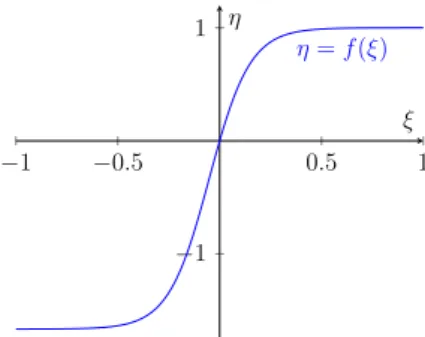
If we restrict our examinations only to positive solutions, then we can apply the transformationx= logy−logK. Thereby we obtain the equation x0(t) =−f(x(t−τ)), (3.1) where the feedback function f ∈C1(R,R)is dened as
f(x) =p− q r+q
p−r
enx for allx∈R, (3.8) see Fig. 3.1. Then we focus on those periodic solutions which oscillate slowly about 0 (SOP solutions), i.e. on those periodic solutions which has zeros spaced at distances greater thanτ.
Nussbaum veried the global existence of SOP solutions for equations of the form (3.1) and for a wide class of feedback functions containing (3.8), see [7] and also [8]. By [7, 8], equation (3.1) has at least one SOP solution for
τ > τ0= π
2f0(0) = qπ 2np(q−pr).
−1 −0.5 0.5 1
−1
1 η=f(ξ)
ξ η
Figure 3.1: The plot off ifp= 1,q= 4, r= 1,5andn= 10
Song, Wei and Han studied the equation in the form (3.6) in [10]. They showed that a series of Hopf bifurcations takes place at the positive equi- librium asτ passes through the critical values
τk = 1 f0(0)
π
2 + 2kπ
= q
np(q−pr) π
2 + 2kπ
, k≥0.
Song and his coauthors could not determine the stability of the periodic orbits for τ far away from the local Hopf bifurcation values. Uniqueness of the slowly oscillatory periodic solution has not been studied either. In the dissertation we focus on these questions and verify the following two theorems.
Theorem 3.8. Set p, q, r andnas in (3.7).
(i) If τ > 0 is large enough, then equation (3.6) has a unique positive periodic solution y¯:R→Roscillating slowly aboutK. The corresponding periodic orbit is asymptotically stable, and it attracts the set
n
φ:yφ(t)>0 fort≥ −τ, ytφ−K has at most one sign change for largeto . (ii) If ω¯ denotes the minimal period ofy¯, and
ω=
2 +q−pr
pr + pr
q−pr
τ, (3.9)
then limτ→∞ω/ω¯ = 1.
Uniqueness of the periodic solution is always meant up to time trans- lation.
If we xp, q, randτ, then we can determine the asymptotic shape of the periodic solution asn→ ∞.
Theorem 3.9. Set p, q, randτ such that (3.7) and τmin{p, q/r−p}>8 hold.
(i) Theorem 3.8.(i) is true for all suciently largen.
(ii) Dene v : R→ R as the ω-periodic extension of the piecewise linear function
[0, ω]3t7→
−pt, 0≤t < τ,
q r−p
t−qrτ, τ≤t <
2 + q−prpr τ,
−pt+q
r+p+q−prp2r
τ,
2 +q−prpr
τ≤t < ω
∈R,
whereω is given by (3.9). Letη1>0 andη2>0be arbitrary. Ifnis large enough, then there exists T ∈ R for the ω¯-periodic solution y¯, such that
|ω¯−ω|< η1, and
logy(t¯ +T) K −v(t)
< η2 for all t∈[0,ω].¯
The proofs of these theorems are similar, and they are organized as follows. We examine equation (3.6) in the form of (3.1) with feedback function (3.8). First we calculate an SOP solutionvfor the "limit equation"
v0(t) =−g(v(t−τ)),
where g : R → R is a piecewise constant function chosen so that (3.8) is close to g outside a neighborhood of 0. Then we consider (3.8) as a perturbation of g and follow the technique used by Walther in [12] (for a slightly dierent class of equations) to obtain information about those solutions of equation (3.1) which has initial segments in
A(β) ={φ∈C: φ(t)≥β for all −τ≤t≤0, φ(0) =β} ⊆C.
We show that these solutions return toA(β)(for appropriately chosenβ).
Thereby a Poincaré-mapP:A(β)→ A(β)can be introduced. Next we ex- plicitly evaluate a Lipschitz constantL(P)forP. Ifτ ornis large enough, then L(P) < 1, i.e., P is a contraction. The unique xed point of P is the initial segment of an SOP solution. Besides this, we need the results of paper [9] of Nussbaum to show that all SOP solutions have segments in A(β), and hence the SOP solution is unique up to time translation. Sta- bility comes from work [1] of Kaplan and Yorke. The rest of the theorems will follow easily.
The details of the proof are described below.
−1 −0.5 0.5 1
−1
1 η=f(ξ)
η=g(ξ)
ξ η
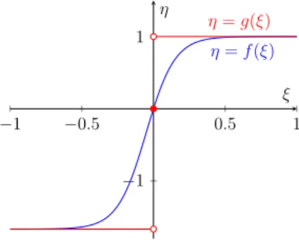
Figure 3.2: The plot ofgA,B
The limit equation
Consider equation (3.1) with feedback function (3.8). LetA=q/r−p >
0 andB=p >0.
Note that ifp, q, rare xed according to (3.7), then f(x)→p−q
r =−A ifnx→ −∞, and
f(x)→p=B ifnx→ ∞.
Therefore in Section 3.3 we examine the "limit equation"
v0(t) =−gA,B(v(t−τ)), (3.11) wheregA,B:R→Ris dened as
gA,B(v) =
−A, v <0, 0, v= 0, B, v >0.
Proposition 3.10. Equation (3.11)admits a periodic solution v:R→R dened as follows:
v(t) =
−Bt, t∈[0, τ],
At−(A+B)τ, t∈[τ, σ+τ],
−Bt+
A+ 2B+BA2
τ, t∈[σ+τ, ω],
whereσ= (1 +B/A)τ is the rst positive zero, andω= (2 +A/B+B/A)τ is the second positive zero and the minimal period ofv.
Preliminary estimates
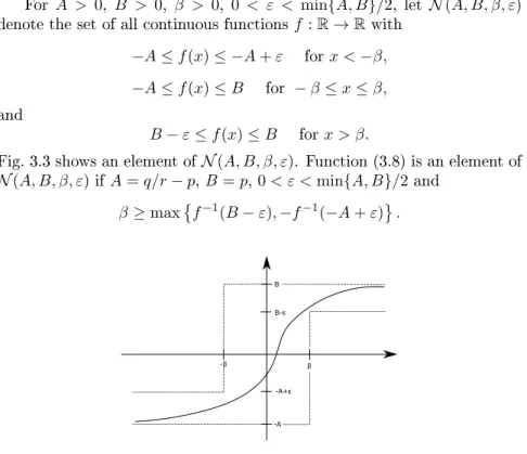
For A > 0, B > 0, β > 0, 0 < ε < min{A, B}/2, let N(A, B, β, ε) denote the set of all continuous functionsf :R→Rwith
−A≤f(x)≤ −A+ε forx <−β,
−A≤f(x)≤B for −β≤x≤β, and
B−ε≤f(x)≤B forx > β.
Fig. 3.3 shows an element ofN(A, B, β, ε). Function (3.8) is an element of N(A, B, β, ε)ifA=q/r−p,B =p,0< ε <min{A, B}/2and
β ≥max
f−1(B−ε),−f−1(−A+ε) .
-A -A+
B- B
-
Figure 3.3: An element ofN(A, B, β, ε)
In Section 3.4 of the dissertation we examine the solutionsx=xφ of the equation (3.1) iff ∈ N(A, B, β, ε)and
φ∈ A(β) ={φ∈C: φ(t)≥β for all −τ≤t≤0,φ(0) =β} ⊆C.
We prove that ifβ andεare chosen correctly, then there areq=q(φ)>0 andq˜= ˜q(φ)such that
xq∈ −A(β) ={φ∈C:φ(t)≤ −β if −τ ≤t≤0, φ(0) =−β}, andxq+˜q ∈ A(β).
We can prove that xq ∈ −A(β) and xq+˜q ∈ A(β) for some q,q >˜ 0 by giving estimates for the
xφ−v
, where v is special periodic function constructed in the previous section. This technique is based on Walther's paper [12].
Lipschitz continuous return maps
Based on the results of the previous section, we can introduce the Poincaré- mapP :A(β)→ A(β). The next step is to determine a Lipschitz constant forP, see Section 3.5 of the dissertation.
Suppose in addition that f ∈ N(A, B, β, ε) is Lipschitz-continuous, and L(f) is a Lipschitz constant for f. Let Lβ = Lβ(f) and L−β = L−β(f)be the Lipschitz constants for the restrictionsf|[β,∞)andf|(−∞,−β], respectively.
In this sectionΦdenotes the semiow corresponding to (3.1):
Φ : [0,∞)×C3(t, φ)7→xφt ∈C.
Consider the map
R:A(β)3φ7→Φ(q(φ), φ) =xφq(φ)∈ −A(β).
Choseεandβ as in the previous section. Then the following is true.
Corollary 3.20. The constant
L(R) = 3τ Lβ(1 +δL(f)) 1 + (N−1)τ L−β(1 +τ L−β)N−2 is a Lipschitz constant for R, where N=d1 +B/Aeandδ= 2β/(B−ε).
Now consider the map
Q:−A(β)3φ7→Φ(˜q(φ), φ)∈ A(β).
It is clear that P=Q◦R. Proposition 3.21. The constant
L(Q) = 3τ L−β
1 + ˜δL(f) 1 + ( ˜N−1)τ Lβ(1 +τ Lβ)N˜−2 is a Lipschitz constant for Q, whereN˜ =d1 +A/Beand˜δ= 2β/(A−ε).
As a consequence, the following can be stated.
Proposition 3.22. The Poincaré map P :A(β)3φ7→Q(R(φ))∈ A(β) is Lipschitz continuous, and
L(P) =L(R)L(Q)
=3τ Lβ(1 +δL(f)) 1 + (N−1)τ L−β(1 +τ L−β)N−2
×3τ L−β
1 + ˜δL(f) 1 + ( ˜N−1)τ Lβ(1 +τ Lβ)N˜−2 . is a Lipschitz constant for P.
IfL(P)<1, then P is a contraction andP has only one xed point, which is the initial segment of a slowly oscillatory periodic solution.
On the ranges of the SOP solutions
In Section 3.6 we show that ifτ is large enough andβ is small enough, then any SOP solutionx:R→Rof (3.1) has segments inA(β).
As we are going to apply paper [9] of Nussbaum, we consider equation (3.1) in form
˜
x0(t) =−τ f(˜x(t−1)), (3.33) wherex(t) =˜ x(τ t)andf is given in (3.8). Set
d=1
2min{−f(−1), f(1), f0(0)}.
In [9] Nussbaum gives specic estimates for the ranges of the slowly oscillatory periodic solutions on dierent subintervals of a real line. The immediate consequence of these estimates is the following proposition.
Proposition 3.26. Ifτ d >4andB is an upper bound forf, then for each SOP solution x˜ :R→Rof (3.33), one can give an interval I of length 1 such that
˜
x(t)≥ τ(√
B2+d2−B)
2 for t∈I.
Corollary 3.27. If τ d > 4 and β ≤τ(√
B2+d2−B)/2, whereB is an upper bound for f, then any SOP solution of (2.2) has a segment inA(β).
Proofs of the main theorems in this chapter
The proof of Theorem 3.8 is the following. We show that ε and β can be chosen such that the propositions described in the previous sections of the dissertation are satised: let ε be a xed, small positive number, and let β =ατ, where α > 0 is also a xed small number. Then for all suciently largeτ,L(P)<1, i.e.,P is a contraction, and the assumptions of Consequence 3.27 are also satised. From this we obtain the existence and uniqueness of the slowly oscillatory periodic solution. Stability follows from Theorem 2.1 and Remark 2.5 of Kaplan and Yorke's paper [1]. The statement for the minimal period of a slowly oscillatory periodic solution is obtained from Theorem 1 of [9].
Theorem 3.9 can be proved in a similar way. The statement describing the asymptotic form of the periodic solution comes immediately from the estimates given for
xφ−v
in Section 3.4.
References
[1] J. L. Kaplan and J. A. Yorke, On the stability of a periodic solution of a dierential delay equation, SIAM J. Math. Anal. 6 (1975), 268282.
[2] T. Krisztin and G. Vas, Large-amplitude periodic solutions for dierential equa- tions with delayed monotone positive feedback, J. Dynam. Dierential Equations, 23 (2011), 727790.
[3] T. Krisztin and G. Vas, The Unstable Set of a Periodic Orbit for Delayed Positive Feedback, J. Dynam. Dierential Equations, 28 (2016), 805855.
[4] A. López Nieto, Periodic orbits of delay equations with monotone feedback and even-odd symmetry, https://arxiv.org/abs/2002.01313
[5] J. Mallet-Paret and G. R. Sell, The Poincaré-Bendixson theorem for monotone cyclic feedback systems with delay, J. Dierential Equations, 125 (1996), no. 2, 441489.
[6] V. G. Nazarenko, Inuence of delay on auto-oscillations in cell populations, Biosika 21 (1976), 352356.
[7] R. D. Nussbaum, Periodic solutions of some nonlinear autonomous functional dierential equations , Ann. Mat. Pura Appl. 101 (1974), 263306.
[8] R. D. Nussbaum, A global bifurcation theorem with applications to functional dierential equations, J. Funct. Anal. 19 (1975), 319338.
[9] R. D. Nussbaum, The range of periods of periodic solutions ofx0(t) =−αf(x(t− 1)). J. Math. Anal. Appl. 58 (1977), no. 2, 280292.
[10] Y. Song, J. Wei and M. Han, Local and global Hopf bifurcation in a delayed hematopoiesis model, Internat. J. Bifur. ChaosAppl. Sci. Engrg. 14 (2004) 3909 3919.
[11] G. Vas, Congurations of periodic orbits for equations with delayed positive feed- back, J. Dierential Equations, 262 (2017), 18501896.
[12] H.-O. Walther, Contracting return maps for some delay dierential equations, Topics in functional dierential and dierence equations (Lisbon, 1999), Fields Inst. Commun., 29, Amer. Math. Soc., Providence, RI, (2001), 349360.
![Figure 2.2: The plot of p on [-1,0]](https://thumb-eu.123doks.com/thumbv2/9dokorg/842691.43844/7.629.167.459.88.766/figure-the-plot-of-p-on.webp)