Saddle-Node Bifurcation of Periodic Orbits for a Delay Differential Equation

Saddle-Node Bifurcation of Periodic Orbits for a Delay Differential Equation

Szandra Beretka^a, Gabriella Vas^b,∗

aBolyai Institute, University of Szeged, 1 Aradi v. tere, Szeged, Hungary

bMTA-SZTE Analysis and Stochastics Research Group, Bolyai Institute, University of Szeged, 1 Aradi v. tere, Szeged, Hungary

Abstract

We consider the scalar delay differential equation

˙

x(t) =−x(t) +fK(x(t−1))

with a nondecreasing feedback functionfK depending on a parameter K, and we verify that a saddle-node bifurcation of periodic orbits takes place as K varies.

The nonlinearityfK is chosen so that it has two unstable fixed points (hence the dynamical system has two unstable equilibria), and these fixed points remain bounded away from each other asKchanges. The generated periodic orbits are of large amplitude in the sense that they oscillate about both unstable fixed points off_K.

Keywords: Delay differential equation, Positive feedback, Saddle-node bifurcation, Large-amplitude periodic solution

2000 MSC:34K13, 34K18, 37G15

1. Introduction

Numerous scientific works have studied the existence and the bifurcation of periodic orbits for delay differential equations, see the books [1, 2, 3] and the survey paper [4] of Walther. In paper [5], Krisztin gives a detailed summary on known results for equations of the special form

˙

x(t) =−x(t) +fK(x(t−1)), (1.1) where fK is monotone nonlinearity. Hopf-bifurcation is a widely studied phe- nomenon [4]. A well-known example is due to Krisztin, Walther and Wu: peri- odic orbits of (1.1) arise via a series of Hopf-bifurcations for strictly monotone in- creasing nonlinearities, e.g., forfK(x) =Ktanh(x) or forfK(x) =Ktan⁻¹(x)

∗Corresponding author

Email addresses: gszandra@math.u-szeged.hu(Szandra Beretka), vasg@math.u-szeged.hu(Gabriella Vas)

asKincreases, see [6, 7, 8]. Other types of bifurcations involving periodic orbits are rarely studied. An interesting example is given by Walther in [9]: he studies a delay equation coming from a prize model, and he shows the bifurcation of periodic orbits with small amplitudes and with periods descending from infinity.

To the best of the authors’ knowledge, no one has verified saddle-node bifurca- tion of periodic orbits for equation (1.1). L´opez Nieto has an analogous result for another class of delay differential equations [10].

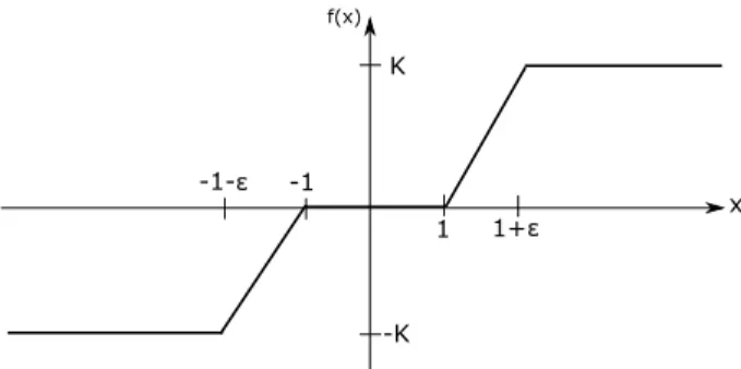
In this paper we consider (1.1) in the so-called positive feedback case;f_K is supposed to be a nondecreasing continuous function such that

fK|_{(−∞,−1−ε]}=−K, fK|_[−1,1] = 0 and fK|_[1+ε,∞)=K,

where ε is a fixed positive number and K is the bifurcation parameter. For technical simplicity, we definefK to be a piecewise linear continuous function:

fK(x) =K

ε (x+ 1) forx∈(−1−ε,−1), and

f_K(x) = K

ε (x−1) forx∈(1,1 +ε), see Fig. 1.1.

The results of the paper are expected to hold if the nondecreasing continuous functionf_K is defined differently on (−1−ε,−1)∪(1,1 +ε), or if the coefficient of the linear term on the right hand side of (1.1) is−µwithµ >0.

The phase space for (1.1) is the Banach space C =C([−1,0],R) with the maximum norm. If for somet ∈R, the interval [t−1, t] is in the domain of a continuous functionx, then the segmentxt∈C is defined byxt(s) =x(t+s) for−1≤s≤0.

If K > 1 +ε, then fK has two fixed points χ₋ ∈ (−1−ε,−1) and χ+ ∈ (1,1 +ε) withf_K⁰ (χ₋)>1 andf_K⁰ (χ+)>1. Thus the constant elements

[−1,0]3s7→χ−∈Rand [−1,0]3s7→χ+∈R

K

-K 1 -1

1+

-1-

x f(x)

Figure 1.1: The plot offK.

ofC are unstable equilibria. We know that there exist periodic solutions oscil- lating about eitherχ−orχ+ifKis sufficiently large, and these periodic orbits appear via Hopf-bifurcations [11].

We say that a periodic solution has large amplitude if it oscillates about bothχ− and χ+. The corresponding orbit is a large-amplitude periodic orbit.

The existence of a pair of large-amplitude periodic orbits has been first shown in [12] for a similar nonlinearityf_K with K large enough. More complicated configurations of such periodic orbits has appeared in [13]. A third work in this topic, the paper [14] has described the complicated geometric structure of the unstable set of a large-amplitude periodic orbit in detail. These works have not explained how these periodic orbits bifurcate as the parameterK changes.

Apparently they cannot appear via Hopf bifurcation in a neighborhood of an unstable equilibrium. In this paper we verify that for the nonlinearityfKdefined above, large-amplitude periodic orbits arise via a saddle-node bifurcation. The following theorem has already appeared in [12] as a conjecture.

Theorem 1.1. (Saddle-node bifurcation of periodic orbits) For all sufficiently small positive ε, one can give a threshold parameter K^∗ = K^∗(ε) ∈ (6.5,7), a large-amplitude periodic solution p = p(ε) : R → R of (1.1) for parameter K=K^∗, an open neighborhood B =B(ε) of its initial segmentp0 in C, and a constantδ=δ(ε)>0 such that

(i) ifK∈(K^∗−δ, K^∗), then no periodic orbit for (1.1) has segments inB;

(ii) ifK=K^∗, thenO={pt:t∈R}is the only periodic orbit with segments inB;

(iii) if K ∈ (K^∗, K^∗+δ), then there are exactly two periodic orbits with segments inB, and both of them are of large-amplitude.

LetK0be that solution of equation

(K−1) (K+ 1)³=e K²−2K−1²

(1.2) that belongs to the interval (6.5,7). It is easy to show thatK0 is unique, see Section 3 of [12]. Numerical computation shows thatK0 ≈6.87. We will see that the limit of the bifurcation parameterK^∗(ε) isK0as ε→0⁺.

The proof is organized as follows. Letε∈(0,1). In Section 2 we introduce a one-dimensional mapF depending also on parametersK andε. In Section 3 we show that the fixed points ofF(·, K, ε) determine large-amplitude periodic solutions for equation (1.1). Then we show in Section 4 that F undergoes a saddle-node bifurcation asKvaries if εis a fixed and sufficiently small positive number. We also need to show that – locally – all periodic solutions can be obtained as fixed points of F(·, K, ε). This is done Section 5. Theorem 1.1 immediately follows from these results, see Section 6. The Appendix contains certain lengthy but straightforward calculations used in Section 4.

In the saddle-node bifurcation ofF, a neutral fixed point splits into two fixed points, one attracting and one repelling. This does not imply that we have one stable and one unstable periodic orbit forK > K^∗. We know that if fK is a C¹-function with nonnegative derivative, then all periodic orbits are unstable,

see e.g., Proposition 7.1 in [13]. Hence we presume that the periodic orbits given by the above theorem are also unstable.

In the previous paper [12], we obtained large-amplitude periodic solutions also as fixed points of finite dimensional maps. We emphasize that here we construct F in a different way. The current approach is simpler because it yields shorter calculations. The advantage of the construction used in [12] is the following: the eigenvalues of the derivatives of the finite dimensional maps in [12] at the fixed points coincide with the Floquet multipliers of the corresponding periodic orbits. Hence those finite dimensional maps give precise information on the stability properties of the periodic orbits. This is not true here.

The reader may find other examples, in which the existence of a periodic orbit is shown by handling a finite dimensional fixed point problem, in the papers [15, 16, 17].

2. The map F

Letε∈(0,1) andK∈(6.5,7). In this section we define a periodic function pas the concatenation of certain auxiliary functions y1, y2, ..., y10 such that if pis a solution of the delay equation (1.1), then y₁, y₂, ..., y₁₀ satisfy a system of ordinary differential equations with boundary conditions. Then we reduce this ODE system to a single fixed point equation of the formF(L₂, K, ε) =L₂, whereL₂ is a parameter corresponding top.

Assume that

(H1) L_i>0 for i∈ {1,2, ...,5},

(H2) 2L₁+ 5L₂+ 5L₃+ 3L₄+ 3L₅= 1,

(H3) θ_i>1 +εfori∈ {1,2,3,4}, andθ_i∈(1,1 +ε) fori∈ {5,6}.

Consider the subsequent continuous functions:

(H4) y1∈C([0, L1],R) withy1(0) = 1 +εandy1(L1) =θ1, y2∈C([0, L2],R) withy2(0) =θ1andy2(L2) =θ2, y3∈C([0, L3],R) withy3(0) =θ2andy3(L3) =θ3, y₄∈C([0, L₄],R) withy₄(0) =θ₃andy₄(L₄) =θ₄, y₅∈C([0, L₅],R) withy₅(0) =θ₄andy₅(L₅) = 1 +ε, y₆∈C([0, L₂],R) withy₆(0) = 1 +εandy₆(L₂) =θ₅, y₇∈C([0, L₃],R) withy₇(0) =θ₅andy₇(L₃) =θ₆, y₈∈C([0, L₄],R) withy₈(0) =θ₆andy₈(L₄) = 1,

y9∈C([0, L2+L5],R) withy9(0) = 1 andy9(L2+L5) =−1, y10∈C([0, L3],R) withy10(0) =−1 andy10(L3) =−1−ε,

(H5) if i∈ {1,2, ...,5}, thenyi(s)>1 +εfor all s in the interior of the domain ofyi,

ifi∈ {6,7,8}, thenyi(s)∈(1,1 +ε) for all sin the interior of the domain ofyi,

y9(s)∈(−1,1) for alls∈(0, L2+L5), y10(s)∈(−1−ε,−1) for alls∈(0, L3).

Fig. 2.1 plots certain horizontal translations ofy1, ..., y10. Set 0< τ1< τ2< τ3< ω <1 as

τ₁=

5

X

i=1

L_i,

τ2=τ1+L2+L3+L4, (2.1) τ₃=τ₂+L₂+L₅,

ω=τ3+L3.

Introduce a 2ω-periodic functionp:R→R as follows. Setp on [−1,−1 +ω]

such that

p(t−1) =y₁(t) fort∈[0, L₁], p(t−1 +L1) =y2(t) fort∈[0, L2], p(t−1 +L₁+L₂) =y₃(t) fort∈[0, L₃], p(t−1 +L1+L2+L3) =y4(t) fort∈[0, L4],

p(t−1 +L1+L2+L3+L4) =y5(t) fort∈[0, L5], (P.1) p(t−1 +τ1) =y6(t) fort∈[0, L2],

p(t−1 +τ1+L2) =y7(t) fort∈[0, L3], p(t−1 +τ₁+L₂+L₃) =y₈(t) fort∈[0, L₄],

p(t−1 +τ2) =y9(t) fort∈[0, L2+L5], p(t−1 +τ₃) =y₁₀(t) fort∈[0, L₃].

Let

p(t) =−p(t−ω) for allt∈[−1 +ω,−1 + 2ω]. (P.2) Then extendpto the real line 2ω-periodically. See Fig. 2.1 for the plot ofp on [−1,1]. It is clear thatpis of large amplitude.

Our first goal is to find what conditions hold for L1, ..., L5, θ1, ..., θ6 and y1, ..., y10 ifpsatisfies equation (1.1) for allt ∈R. As p(t) =−p(t−ω) for all realtandfK is odd, we do not lose information if we restrict our examinations to the interval [0, ω]. So consider

˙

p(t) =−p(t) +f_K(p(t−1)) fort∈[0, ω]. (2.2) We study (2.2) first on the interval [0, τ₁], then on [τ₁, τ₂], [τ₂, τ₃] and [τ₃, ω].

1. The interval [0, τ₁]. The way we extended pfrom [−1,−1 +ω] toRand condition (H2) together imply that

p(t) =−y8(t) fort∈[0, L4], p(t+L4) =−y9(t) fort∈[0, L2+L5], p(t+L4+L2+L5) =−y10(t) fort∈[0, L3], p(t+L₄+L₂+L₅+L₃) =y₁(t) fort∈[0, L₁],

see Fig. 2.1. Also observe – using (P.1) and (H3)-(H5) – that p(t)≥1 +ε fort∈[−1,−1 +τ1],

and thus (2.2) is in the form ˙p(t) =−p(t) +Kon [0, τ1]. We conclude that (2.2) holds fort∈[0, τ₁] if and only if the subsequent four equations are satisfied:

˙

y₈(t) =−y₈(t)−K, t∈[0, L₄], (2.3)

˙

y9(t) =−y9(t)−K, t∈[0, L2+L5], (2.4)

˙

y₁₀(t) =−y₁₀(t)−K, t∈[0, L₃], (2.5)

˙

y1(t) =−y1(t) +K, t∈[0, L1]. (2.6) 2. The interval[τ₁, τ₂].By the definition ofpand hypothesis (H2),

p(t+τ₁) =y₂(t) fort∈[0, L₂], p(t+τ1+L2) =y3(t) fort∈[0, L3] and

p(t+τ1+L2+L3) =y4(t) fort∈[0, L4].

We also know from (P.1) that

p(t−1 +τ₁) =y₆(t) fort∈[0, L₂], p(t−1 +τ1+L2) =y7(t) fort∈[0, L3], p(t−1 +τ₁+L₂+L₃) =y₈(t) fort∈[0, L₄].

Hypotheses (H3)-(H5) then guarantee that

p(t)∈[1,1 +ε] fort∈[−1 +τ1,−1 +τ2].

Using the definition offK, we obtain that (2.2) holds on [τ1, τ2] if and only if

˙

y₂(t) =−y₂(t) +K

ε (y₆(t)−1) fort∈[0, L₂], (2.7)

˙

y3(t) =−y3(t) +K

ε (y7(t)−1) fort∈[0, L3] (2.8) and

˙

y4(t) =−y4(t) +K

ε(y8(t)−1) fort∈[0, L4]. (2.9) 3. The interval [τ2, τ3].Next observe that

p(t+τ2) =y5(t) fort∈[0, L5], p(t+τ2+L5) =y6(t) fort∈[0, L2] and

p(t)∈[−1,1] fort∈[−1 +τ2,−1 +τ3].

Therefore

˙

y5(t) =−y5(t) fort∈[0, L5] (2.10) and

˙

y6(t) =−y6(t) fort∈[0, L2]. (2.11) 4. The interval [τ₃, ω].At least observe that

p(t+τ₃) =y₇(t) fort∈[0, L₃], p(t−1 +τ3) =y10(t) fort∈[0, L3], and

p(t)∈[−1−ε,−1] fort∈[−1 +τ3,−1 +ω].

So on the interval [τ₃, ω], equation (2.2) is equivalent to

˙

y7(t) =−y7(t) +K

ε (y10(t) + 1), t∈[0, L3]. (2.12) We see that under hypotheses (H1)-(H5), equation (2.2) is equivalent to a system of linear ordinary differential equations. It worth solving equations (2.3)-(2.6) and (2.10)-(2.11) first because they are independent from the other ones. Then we can solve (2.7), (2.9) and (2.12) using the solutions of (2.11), (2.3) and (2.5), respectively. At last, using the solution of (2.12), we can find the solution of (2.8). Applying the boundary conditions given by (H4) fort= 0, we obtain that

y₁(t) =K−(K−1−ε)e^−t, t∈[0, L₁], (Y.1) y2(t) =θ1e^−t+K

ε (1 +ε)te^−t+e^−t−1

, t∈[0, L2], (Y.2) y3(t) =θ2e^−t+K

ε (θ5t+ 1)e^−t−1

(Y.3)

−K²

ε² (K−1)

1−

1 +t+t² 2

e^−t

, t∈[0, L3], y4(t) =θ3e^−t+K

ε (K+θ6)te^−t−(K+ 1) 1−e^−t

, t∈[0, L4], (Y.4)

y₅(t) =θ₄e^−t, t∈[0, L₅], (Y.5)

y₆(t) = (1 +ε)e^−t, t∈[0, L₂], (Y.6)

y7(t) =θ5e^−t−K

ε(K−1) 1−(1 +t)e^−t

, t∈[0, L3], (Y.7) y8(t) = (K+θ6)e^−t−K, t∈[0, L4], (Y.8) y9(t) = (K+ 1)e^−t−K, t∈[0, L2+L5], (Y.9) y10(t) = (K−1)e^−t−K, t∈[0, L3]. (Y.10)

If we apply the boundary conditions given for the right end points of the domains ofyi, i∈ {1, ...,10}, then we get the following relations:

θ₁=K−(K−1−ε)e^−L1, (B.1)

θ2=θ1e^−L2+K

ε (1 +ε)L2e^−L2+e^−L2−1

, (B.2)

θ3=θ2e^−L3+K

ε (θ5L3+ 1)e^−L3−1

(B.3)

−K²

ε² (K−1)

1−

1 +L3+L²₃ 2

e^−L3

, θ4=θ3e^−L4+K

ε (K+θ6)L4e^−L4−(K+ 1) 1−e^−L4

, (B.4)

1 +ε=θ4e^−L5, (B.5)

θ5= (1 +ε)e^−L2, (B.6)

θ₆=θ₅e^−L3−K

ε (K−1) 1−(1 +L₃)e^−L3

, (B.7)

1 = (K+θ6)e^−L4−K, (B.8)

−1 = (K+ 1)e^−L2−L5−K, (B.9)

−1−ε= (K−1)e^−L3−K. (B.10)

Next we reduce the algebraic system of equations (H2), (B.1)-(B.10) to a single equation for L2, K and ε. Meanwhile, we express L1, L3, L4, L5 and θ1, θ2, ..., θ6 as functions ofL2, K andε.

By (B.10),

L₃= ln K−1

K−1−ε. (C.1)

From (B.9) and (B.5) we obtain that L₅= lnK+ 1

K−1 −L₂ (C.2)

and

θ₄= (1 +ε)K+ 1

K−1e^−L2. (C.3)

θ5 is already expressed in (B.6). In order to simplify reference to the formulas in this section, we repeat that

θ₅= (1 +ε)e^−L2. (C.4)

Using this, (B.7) and (C.1), we calculate that θ₆= (1 +ε)K−1−ε

K−1 e^−L2+K

ε(K−1−ε) ln K−1

K−1−ε−K. (C.5) Note thatθ₆+K >0. From (B.8) we obtain that

L4= lnK+θ6

K+ 1. (C.6)

Now we use (H2), (C.1) and (C.6) to expressL1: L1= 1

2−L2+5

2ln (K−1−ε)−3

2ln (K+θ6)−ln (K−1). (C.7) Substituting the last relation into (B.1), we get that

θ₁=K−e^L2−12(K−1) (K+θ₆)³²

(K−1−ε)³² . (C.8)

Then replacingθ1by (C.8) in (B.2), we conclude that θ2=Ke^−L2−e⁻¹²(K−1)(K+θ₆)³²

(K−1−ε)³² +K

ε (1 +ε)L2e^−L2+e^−L2−1 . (C.9) Parameterθ3 appeared as a function of K, ε, θ2, θ5 andL3 in (B.3). As θ2, θ5

andL3 have already been given as functions ofL2, K andε, now we see thatθ3

can also be expressed as a function ofL2, K and ε. We will considerθ3 in the form

θ3=θ2e^−L3+K

ε (1 +ε)L3e^−L2−L3+e^−L3−1

(C.10)

−K²

ε² (K−1)

1−

1 +L₃+L²₃ 2

e^−L3

, whereθ₂ andL₃are defined by (C.9) and (C.1), respectively.

Then (B.4) is the only algebraic equation we have not used so far. We substitute (C.3) into the left hand side of (B.4) and then multiply this equation bye^L4= (K+θ₆)/(K+ 1). We deduce that

(1 +ε)K+θ₆

K−1 e^−L2 =K

ε(K+ 1) 1−(1−L₄)e^L4 +θ₃. Let

U =

(L2, K, ε)∈R³: ε∈(0,1), K ∈(6.5,7), L2∈(−ε, ε) .

If we considerθ₃, θ₆andL₄as functions onU given by (C.10), (C.5) and (C.6), then we can define a mapF :U →Rby

F(L2, K, ε) = K

ε(K+ 1) 1−(1−L4)e^L4

+θ3−(1 +ε)K+θ₆

K−1e^−L2+L2

for all (L2, K, ε)∈U. One can easily check thatF is well-defined and continuous onU.

The following proposition holds.

Proposition 2.1. Let ε∈(0,1) andK∈(6.5,7). Suppose that p:R→Ris a 2ω-periodic solution of (1.1),pis the concatenation of functionsy1, y2, . . . , y10

as given in (P.1)-(P.2), furthermore the functions y1, y2, . . . , y10 satisfy (H1)- (H5) with some parametersLi>0,i∈ {1,2, ...,5}, andθi,i∈ {1, . . . ,6}. Then L2∈(0, ε)andF(L2, K, ε) =L2.

Proof. Recall from (C.4) thatθ5= (1 +ε)e^−L2, which is greater than 1 by (H3).

It follows immediately thatL2<ln (1 +ε)< ε. The rest of the statement comes from the above calculations.

We need to considerF also forL2∈(−ε,0] because of technical reasons; see Proposition 4.2 in Section 4. We will also use the following remark in the next section.

Remark 2.2. The system of algebraic equationsF(L₂, K, ε) =L₂, (C.1)-(C.10) is equivalent to the system of equations (H2), (B.1)-(B.10).

3. The fixed points of F yield periodic solutions

By the previous section, if (H1)-(H5) hold, andp:R→Ris a 2ω-periodic so- lution of (1.1) given by (P.1)-(P.2), thenL₂7→F(L₂, K, ε) has a fixed point. We devote this section to verify the converse statement: ifε >0 is small enough and K∈(6.5,7), then all sufficiently small positive fixed points ofL₂7→F(L₂, K, ε) yield periodic solutions of (1.1).

We need to consider L1, L3, L4, L5 andθi, 1≤i≤6, as functions ofL2, K andε(and not as parameters given by hypotheses (H1)-(H5)). So assume that (H6) Li,i∈ {1,3,4,5}, andθi,1≤i≤6, are defined by (C.1)-(C.10) on

U =

(L2, K, ε)∈R³: ε∈(0,1), K∈(6.5,7) andL2∈(−ε, ε) . One easily check that Li, i ∈ {1,3,4,5}, and θi, 1 ≤ i ≤ 6, are continuous functions of (L2, K, ε) onU.

In this section we also need the assumption that

(H7) y₁, ..., y₁₀ are the solutions (Y.1)-(Y.10) of the ordinary differential equations (2.3)-(2.12).

Set

θ^∗ K¯

= ¯K− v u u t

K¯ + 1³

e K¯ −1 for ¯K∈[6.5,7]. We claim thatθ^∗ K¯

>1 for ¯K∈[6.5,7]. As this inequality is equivalent to

K¯ −1



1− v u u t

K¯ + 13

e K¯ −13



>0, we need to verify that K¯ + 1³

/ K¯ −1³

< e holds. Indeed, since ¯K 7→

K¯ + 1

/ K¯ −1

is strictly decreasing for ¯K >1, we see that K¯ + 1

K¯ −1 ³

≤

6.5 + 1 6.5−1

3

= 15

11 3

= 2 + 713

1331 ≤2 + 800

1200 = 2 +2

3 < e (3.1)

for ¯K∈[6.5,7].

The first two statements of the subsequent proposition give information on the behavior ofF for small positiveε. The third statement examines the limit ofy2(t),y3(t) andy4(t) for alltin their domains asε→0⁺. Sincey2,y3andy4

are well-defined by (Y.2)-(Y.4) only ifLi ≥0 fori∈ {2,3,4}, here we assume that L₂ ≥0 and L₄ ≥0. It is clear that L₃ = ln(K−1)−ln(K−1−ε) is positive.

Proposition 3.1. The subsequent assertions hold under hypothesis (H6).

(i)θ₆= 1 +O(ε),L₄=O(ε)and thus K

ε(K+ 1) 1−(1−L4)e^L4

=O(ε) asε→0⁺. (ii) IfK→K¯ ∈[6.5,7]andε→0⁺, thenθ3 converges toθ^∗ K¯

.

(iii) Assume in addition thatL2≥0andL4≥0. Definey2,y3andy4by (Y.2)- (Y.4). IfK →K¯ ∈[6.5,7] andε→0⁺, then y2(t), y3(t)and y4(t) converges toθ^∗ K¯

, uniformly int∈[0, L2],t∈[0, L3]andt∈[0, L4], respectively.

Before giving the proof of this proposition, let us make a remark on notation O. If g is a function ofL2, K, ε, t(or only some of these variables) on a setD, andkis a positive integer, then the expressiong=O ε^k

asε→0⁺(or simply g=O ε^k

) means that there exists M >0 such that |g(L2, K, ε, t)| ≤M ε^k if (L2, K, ε, t)∈D and ε >0 is sufficiently close to zero. Constant M is always independent fromL2, K andt in this paper.

Proof. The proof of statement (i). It is well-known that ln(1 +x) =x+O x²

as x→0. (3.2)

IfK∈(6.5,7) andε→0⁺, then ε

K−1−ε→0⁺ and thus

ln K−1 K−1−ε = ln

1 + ε

K−1−ε

= ε

K−1−ε+O ε²

asε→0⁺. (3.3) Therefore

K

ε(K−1−ε) ln K−1

K−1−ε =K+O(ε). (3.4) In addition, sinceL2∈(−ε, ε),

(1 +ε)K−1−ε

K−1 e^−L2 = (1 +ε)

1− ε K−1

(1 +O(L2)) = 1 +O(ε). (3.5) Substituting (3.4) and (3.5) into (C.5), we obtain thatθ₆= 1 +O(ε).

Using (C.6), the previous statement regardingθ6and (3.2), we immediately get that

L4= ln

1 +θ6−1 K+ 1

=O(ε). (3.6)

By the power series expansion of the exponential function, 1−e^L4(1−L4) =O L²₄

as L4→0. (3.7)

The last statement of Proposition 3.1.(i) then comes from (3.6) and (3.7).

The proof of statement (iii). Let us now prove (iii) in three steps. Let L2≥0 andL4≥0.

1. The convergence of y₂(t) for t∈[0, L₂]. We see from statement (i) and formula (C.8) that

lim

K→K¯ ε→0⁺

θ1= ¯K− v u u t

K¯ + 13

e K¯ −1 =θ^∗ K¯

. (3.8)

Using that 0≤t≤L₂< εande^x= 1 +x+O x²

asx→0, we also see that K

ε (1 +ε)te^−t+e^−t−1

= K

ε (1 +ε)t 1−t+O t²

−t+O t²

= K

ε εt+O t²

=O(ε).

(3.9)

Substituting (3.8) and (3.9) into (Y.2), we get thaty2(t) converges to θ^∗ K¯ for allt∈[0, L2],and this convergence is uniform in t.

2. The convergence of y3(t) for t ∈ [0, L3], using formula (Y.3). Observe that if θ1 is given by (C.8), and θ2 is determined by (C.9), then (Y.2) yields thaty2(L2) =θ2. So by our last result, lim_ε→0+,K→K¯θ2=θ^∗ K¯

. We also see from (C.4) and fromL2∈(−ε, ε) thatθ5= 1 +O(ε) asε→0⁺.Using this and the power series expansion of the exponential function, we get the following for 0≤t≤L3=O(ε):

(θ₅t+ 1)e^−t−1 = ((1 +O(ε))t+ 1) 1−t+O t²

−1 =O ε²

. (3.10) We also observe that

1−e^−t

1 +t+t² 2

=1−

1−t+t²

2 +O(t³) 1 +t+t² 2

=O ε³ .

(3.11)

Summing up, (Y.3) yields that if 0≤t≤L3=O(ε), then lim

K→K¯ ε→0⁺

y₃(t) = lim

K→K¯ ε→0⁺

θ₂e^−t=θ^∗ K¯ .

This convergence is uniform int.

3. The convergence ofy4(t) fort∈[0, L4]. On the one hand, ify3is defined by (Y.3), θ5 is defined (C.4) and θ3 is given by (C.10), then θ3 = y3(L3).

Hence, by the previous paragraph,θ3 converges toθ^∗ K¯

if K→K¯ ∈[6.5,7]

andε→0⁺. (Note that we have proved statement (ii) in the caseL2≥0). On the other hand, it follows fromθ6= 1 +O(ε) that

(K+θ₆)te^−t−(K+ 1) 1−e^−t equals

(K+ 1 +O(ε)) t+O t²

−(K+ 1) t+O t²

=O ε²

for 0≤t≤L4=O(ε). In consequence, formula (Y.4) shows thaty4(t) converges toθ^∗ K¯

, uniformly int∈[0, L4].

The proof of statement (ii). We have already verified (ii) for L2 ∈ [0, ε).

Now suppose that L2 ∈ (−ε,0) and observe that (3.9) holds also with t = L2 ∈ (−ε,0). Therefore (C.9) and the equality θ6 = 1 +O(ε) together show that θ2 converges to θ^∗ K¯

also in the case when L2 < 0. Now we can use L3 =O(ε), (C.4) and (3.10)-(3.11) with t = L3 to verify that θ3 (defined by (C.10)) converges toθ^∗ K¯

ifK→K¯ ∈[6.5,7],ε→0⁺ andL2∈(−ε,0).

Corollary 3.2. Assume thatlim_n→∞ε_n= 0⁺,

(L_2,n, K_n, ε_n)∈U and F(L_2,n, K_n, ε_n) =L_2,n for alln≥0.

Then (K_n)^∞_n=0 is convergent, and lim_n→∞K_n = K₀, where K₀ is the unique solution of (1.2) in [6.5,7].

Proof. We already know from Section 3 of paper [12] that (1.2) has exactly one solutionK0≈6.87 in [6.5,7].

It suffices to prove that each subsequence of (Kn)^∞_n=0 has a subsequence converging toK0. AsKn∈(6.5,7) for alln≥1, it is clear that any subsequence of (Kn)^∞_n=0has a convergent subsequence (Kn_l)^∞_l=0. Let

K¯ = lim

l→∞Kn_l∈[6.5,7].

Now letltend to infinity in the equationF(L2,n_l, Kn_l, εn_l) =L2,n_l. Under the assumptions of the Corollary, lim_l→∞L_2,nl = 0. This fact, the definition of F and Proposition 3.1.(i)-(ii) together show that ¯K∈[6.5,7] is a solution of

K− s

(K+ 1)³

e(K−1) −K+ 1 K−1 = 0.

It is straightforward to show that this equation is equivalent to (1.2), and thus K¯ =K0. The proof is complete.

ForK∈(6.5,7) and ε∈(0,1), letLb2 be that value ofL2 for whichL4= 0, i.e., for whichθ6= 1.Using (C.5), we can expressLb2 as a function ofKandε:

Lb₂(K, ε) = ln

(1 +ε)K−1−ε K−1

−ln

K+ 1−K

ε(K−1−ε) ln K−1 K−1−ε

.

(3.12)

Proposition 3.3. If K∈(6.5,7) andε >0 is small enough, then Lb2(K, ε)∈ (0, ε).

Proof. It is well-known that

ln(1 +x) =x−x²

2 +O x³

asx→0.

In consequence, ln K−1

K−1−ε = ln

1 + ε

K−1−ε

= ε

K−1−ε− ε²

2(K−1−ε)²+O ε³ , and

K

ε (K−1−ε) ln K−1

K−1−ε =K− Kε

2(K−1−ε)+O ε²

as ε→0⁺. (3.13) Applying the geometric series expansion (1−x)⁻¹=P∞

n=0xⁿ with the choice x=ε/(K−1), we easily deduce that

1

K−1−ε= 1

K−1 · 1

1−_K−1^ε = 1

K−1+O(ε), and thus

K

ε(K−1−ε) ln K−1

K−1−ε =K− K

2(K−1)ε+O ε²

. (3.14)

Using this, we get that ln

K+ 1−K

ε(K−1−ε) ln K−1 K−1−ε

= K

2(K−1)ε+O ε²

. (3.15) Also note that

(1 +ε)K−1−ε

K−1 = 1 + K−2

K−1ε− 1 K−1ε², and thus

ln

(1 +ε)K−1−ε K−1

= K−2

K−1ε+O ε²

. (3.16)

Subtracting (3.15) from (3.16), we conclude that Lb2=

K−2

K−1 − K 2(K−1)

ε+O ε²

= K−4

2(K−1)ε+O ε²

. (3.17) Since (K−4)/(2K−2)∈(0,1) for K∈(6.5,7), we see thatLb2∈(0, ε) for all sufficiently small positiveε.

Consider the following subset ofU: V =n

(L₂, K, ε) : ε∈(0,1), K∈(6.5,7) andL₂∈

0,Lb₂(K, ε)o

⊂U.

Remark 3.4. It is clear from (C.5) and (C.6) thatθ6andL4are strictly decreas- ing functions of L₂. Hence, if ε > 0 is small and (L₂, K, ε) ∈V, then θ₆ >1 andL₄>0.

Now we are ready to clarify which fixed points of L₂ 7→ F(L₂, K, ε) yield periodic solutions.

Proposition 3.5. Assume that

• (L2, K, ε)∈V,F(L2, K, ε) =L2 andε >0 is sufficiently small,

• L1, L3, L4, L5 andθi,1≤i≤6, are defined as in (H6),

• yi,1≤i≤10, are defined as in (H7).

Then (H1)-(H5) hold.

Proof. The functionsy1, ..., y10can be defined by (Y.1)-(Y.10) only ifL1, L2, L3, L4 and L5 are nonnegative. So let us first show (H1). It is clear from (C.1) that L₃ >0, and we know from Remark 3.4 that L₄ >0. Corollary 3.2 and formula (C.2) yield that if(and henceL₂) tends to 0, thenL₅tends to ln((K₀+ 1)/(K₀−1)). Similarly, Corollary 3.2 and formula (C.7) give that

lim

ε→0⁺L₁=1 2 −1

2ln

K0+ 1 K₀−1

³

This limit is also positive, see (3.1). ThusL1 and L5 are positive if ε > 0 is small enough.

By Remark 2.2, equation F(L2, K, ε) = L2 and (C.1)-(C.10) imply (H2).

Thus (H2) holds under the assumptions of this proposition.

It is clear from (Y.1)-(Y.10) that y1, ..., y10 are continuous. Recall that they are those solutions of the ordinary differential equations (2.3)-(2.12) that satisfy the boundary conditions listed in (H4) for t = 0. In addition, by Re- mark 2.2, equationF(L2, K, ε) =L2and (C.1)-(C.10) imply that the equations (B.1)-(B.10) are true. This means thaty₁, ..., y₁₀satisfy the right-end boundary conditions given in (H4). Summing up, (H4) is satisfied.

It remains to show (H3) and (H5).

AsK−1−εis positive for (L2, K, ε)∈V, we see from (Y.1) thaty1strictly monotone increases on [0, L1]. As y1(0) = 1 +ε, it follows that y1(t)>1 +ε fort∈(1, L1]. Thusθ1=y1(L1)>1 +ε. Using Proposition 3.1.(iii), we obtain that y2(t), y3(t) and y4(t) are greater than 1 +ε for all t if ε > 0 is small enough. It follows immediately thatθ2=y2(L2),θ3=y3(L3) andθ4=y4(L4) are greater than 1 +εifε >0 is small enough. It is clear from (Y.5) thaty₅is strictly monotone decreasing. Asy₅(L₅) = 1 +ε, we deduce thaty₅(t)>1 +ε for t ∈ [0, L₅). Summing up the results of this paragraph, θ_i > 1 +ε for i ∈ {1,2,3,4}, and y_i(t)> 1 +ε for all t in the interior of the domain of y_i, wherei∈ {1,2, . . . ,5}.

By (Y.6) and (Y.8), y6 and y8 are strictly monotone decreasing on their whole domains. Differentiating (Y.7) with respect to t and using that θ5 >0 by (C.4), we conclude that

˙

y7(t) =−θ5e^−t−(1 +K)te^−t<0 fort∈[0, L3], i.e.,y7 is also strictly monotone decreasing on [0, L3]. Hence

1 +ε=y6(0)> y6(L2) =θ5=y7(0)> y7(L3) =θ6=y8(0)> y8(L4) = 1, and y_i(s) ∈ (1,1 +ε) for all s in the interior of the domain of y_i, where i ∈ {6,7,8}.

From (Y.9) and (Y.10) we conclude that y₉ and y₁₀ are strictly monotone decreasing on [0, L₂+L₅] and on [0, L₃], respectively. As we already know thaty₉ andy₁₀ fulfill the boundary conditions given in (H4), it is obvious that y9(t)∈(−1,1) for allt∈(0, L2+L5), andy10(t)∈(−1−ε,−1) for allt∈(0, L3).

We have verified (H3) and (H5), and hence the proof is complete.

Corollary 3.6. Under the assumptions of the previous proposition, the 2ω- periodic functionp, determined by (P.1)-(P.2), satisfies the delay equation (1.1) onR. In addition, the map

V 3(L2, K, ε)7→p0∈C is continuous.

Proof. As p(t) =−p(t−ω) for all real t, and the nonlinearityf_K is odd, it is enough to guarantee (2.2) to prove thatp is a solution onR. By Proposition 3.5, the properties listed in (H1)-(H5) are true. We have already pointed out in Section 2 that – under hypotheses (H1)-(H5)– equation (2.2) is equivalent to the ordinary equations

• (2.3)-(2.6) on [0, τ1],

• (2.7)-(2.9) on [τ1, τ2],

• (2.10)-(2.11) on [τ2, τ3],

• and (2.12) on [τ3, ω].

By assumption (H7), (2.3)-(2.12) hold. So (2.2) is satisfied too.

Recall the observation that under hypothesis (H6), Li, i∈ {1,3,4,5}, and θi, 1 ≤ i ≤ 6, are continuous functions of (L2, K, ε) on V. From this, from the definitions (Y.1)-(Y.10) ofy1, . . . , y10 and from (P.1)-(P.2) one can deduce in a straightforward way that the initial functionp0 varies continuously with (L₂, K, ε). We leave the details to the reader.

4. The saddle-node bifurcation ofF_ε Forε∈(0,1), let

Uε= (−ε, ε)×(6.5,7) and define

F_ε:U_ε3(L₂, K)7→F(L₂, K, ε)∈R.

Appendix A of this paper calculates certain partial derivatives ofF_εand shows that∂F_ε/∂K and∂²F_ε/∂L²₂are both continuous onU_ε. One can actually show thatF_ε∈C²(U_ε). We omit the complete proof of this claim.

In this section we consider ε to be a fixed and sufficiently small positive number and show thatFε undergoes a saddle-node bifurcation asK increases.

The first two propositions show that if L2 ∈ (−ε, ε), then the equation Fε(L2, K) =L2can be solved forK.

Proposition 4.1. If ε >0 is sufficiently small, then there existsKε∈(6.5,7) so thatFε(0, Kε) = 0.

Proof. Using Proposition 3.1, we obtain that for anyK∈(6.5,7), lim

ε→0⁺Fε(0, K) =K− s

(K+ 1)³

e(K−1)−K+ 1

K−1. (4.1)

One can show by elementary calculations that the sign of (4.1) is the same as the sign of

w(K) =e−(K+ 1)³(K−1) (K²−2K−1)², which expression is slightly easier to handle. As

w(6.5) =e−37125

12769 < e−36400

13000 =e−28 10 <0 and

w(7) =e−768

289 > e−768

288 =e−8 3 >0,

one sees that lim_ε→0+Fε(0,6.5) <0 and lim_ε→0+Fε(0,7)>0. Hence, ifε >0 is small enough, then Fε(0,6.5) < 0 and Fε(0,7) > 0. As (6.5,7) 3 K 7→

F_ε(0, K)∈ Ris continuous, the existence of K_ε follows from the intermediate value theorem.

Proposition 4.2. For all sufficiently small positive ε and L2 ∈ (−ε, ε), the equationFε(L2, K) =L2 has a unique solutionK in(6.5,7). Furthermore, this solution can be given asK=ϕε(L2), whereϕε: (−ε, ε)→(6.5,7)is continuous andϕε(0) =Kε.

Proof. LetJε= (6.5−Kε,7−Kε) and introduce the map

G_ε: (−ε, ε)×J_ε3(L₂, K)7→F_ε(L₂, K+K_ε)−L₂∈R.

Then Gε(0,0) = 0 and Gis continuously differentiable (see Propositions A.2 and A.4 in Appendix A). We look for the solutionKofGε(L2, K) = 0 for any smallε >0 and for anyL2∈(−ε, ε).

Let

A:=∂G_ε(0,0)

∂K = ∂F_ε(0, K_ε)

∂K .

By Corollary A.3, we may assume thatAis nonzero.

Finding a solutionK toGε(L2, K) = 0 is equivalent to finding a fixed point ofTε,L₂, where

T_ε,L2 :J_ε3K7→K−A⁻¹G_ε(L₂, K)∈R.

Choose a constantq∈(0,1) independent fromK, εandL2. We claim that Tε,L₂ is a uniform contraction on an appropriate subset of Jε: ifη >0 is small enough, then [−η, η]⊆Jε,

|Tε,L₂(K)| ≤η forK∈[−η, η], (4.2) and

|T_ε,L2(K₁)−T_ε,L2(K₂)|< q|K₁−K₂| forK₁, K₂∈[−η, η]. (4.3) Setη >0 so small that [−η, η]⊆J_ε. Using Lagrange’s mean value theorem, we get that forK₁, K₂∈[−η, η],

|Tε,L₂(K1)−Tε,L₂(K2)|6 sup

|^K¯|^<η

1−A⁻¹∂Gε(L2,K)¯

∂K

|K1−K2|. (4.4)

We see from Proposition A.2 that

∂Gε(L2,K)¯

∂K = 1−e⁻¹²



 3 2

s

Kε+ ¯K+ 1 Kε+ ¯K−1 −1

2 s

Kε+ ¯K+ 1 Kε+ ¯K−1

³





+ 2

(Kε+ ¯K−1)² +O(ε).

(4.5)

Therefore there exist ε0 >0 and η0 >0 such that if ε∈ (0, ε0), L2 ∈(−ε, ε) and ¯K∈(−η0, η0), then

1−A⁻¹∂Gε(L2,K)¯

∂K

< q,

that is, (4.3) is satisfied for anyε∈(0, ε0),L2∈(−ε, ε) andη ∈(0, η0). Next, using the Taylor expansion ofGε, we obtain that

Tε,L2(K) =K−A⁻¹Gε(L2, K) =−A⁻¹

∂G_ε(0,0)

∂L2

L2+O L²₂+K²

asL₂→0 andK→0. In consequence, if|K| ≤η < η₀ and|L₂|< ε < ε₀, then

|Tε,L₂(K)|<|A|⁻¹

∂Gε(0,0)

∂L₂

ε+C ε²+η²

with some constantC > 0. Fix η1 < η0 so small that Cη₁² < η1/2. Now set ε₁< ε₀ such that

|A|⁻¹

∂Gε(0,0)

∂L2

ε+Cε²< η1

2

for allε∈(0, ε1). Then (4.2) holds forη =η1, ε∈(0, ε1) andL2∈(−ε, ε).

Summing up, we conclude thatTε,L₂ is a uniform contraction from [−η1, η1] to [−η1, η1] for all ε ∈ (0, ε1) and L2 ∈ (−ε, ε). By the Banach fixed point theorem, Tε,L₂ has a unique fixed point ψε(L2) in [−η1, η1], see Theorem 3.1 of Chapter 0 in [18]. SinceL27→Tε,L₂(K) is continuous for each K, it follows from Theorem 3.2 of Chapter 0 in [18] that ψε is continuous in L2. It is clear thatψε(0) = 0. Setϕε(K) :=Kε+ψε(K).

Now we are ready to verify the saddle-node bifurcation of the fixed points ofF_ε.

Proposition 4.3. For all sufficiently small positive ε, one can give K^∗ = K^∗(ε)∈(6.5,7)andL^∗₂=L^∗₂(ε)∈(0,Lb2(K, ε))such thatFεundergoes a saddle- node bifurcation at(L^∗₂, K^∗): there exist a neighborhoodU ofL^∗₂in(0,Lb2(K^∗, ε)) and a constantδ1>0such that

• the map Fε(·, K)has no fixed point in U forK∈(K^∗−δ1, K^∗),

• L^∗₂ is the unique fixed point of F_ε(·, K^∗)inU,

• Fε(·, K)has exactly two fixed points inU forK∈(K^∗, K^∗+δ1), and both fixed points converge to L^∗₂ asK→K^∗.

Proof. By Section 21.1A in [19], Fε undergoes a saddle-node bifurcation at (L^∗₂, K^∗) if

F_ε(L^∗₂, K^∗) =L^∗₂,

∂

∂L₂Fε(L^∗₂, K^∗) = 1,

∂

∂KFε(L^∗₂, K^∗)6= 0,

∂²

∂L²₂Fε(L^∗₂, K^∗)6= 0.

Furthermore, if

∂²

∂L²₂F_ε(L^∗₂, K^∗)

∂

∂KFε(L^∗₂, K^∗) <0, then the fixed points ofF_εappear for K≥K^∗.

For all small enough positive ε, Proposition 4.2 gives a continuous map ϕε: (−ε, ε)→(6.5,7) such that

F_ε(L₂, ϕ_ε(L₂)) =L₂ for allL₂∈(−ε, ε).

It is clear from Corollary A.5 that ifε >0 is sufficiently small, then

∂

∂L₂F_ε(0, ϕ_ε(0))>1 and ∂

∂L₂F_ε

Lb₂, ϕ_ε Lb₂

<1.

AsFεis continuously differentiable with respect toL2, andϕ is continuous, it is clear that

(−ε, ε)3L27→ ∂

∂L₂Fε(L2, ϕε(L2))∈R

is also continuous. It follows from the intermediate value theorem that there existsL^∗₂∈(0,Lb2) such that

∂

∂L₂Fε(L^∗₂, ϕε(L^∗₂)) = 1.

LetK^∗:=ϕε(L^∗₂)∈(6.5,7).

We see from Corollary A.3 and from Proposition A.6 that we may assume that

∂

∂KF_ε(L^∗₂, K^∗)>0 and ∂²

∂L²₂F_ε(L^∗₂, K^∗)<0.

Hence Fε undergoes a saddle-node bifurcation at (L^∗₂, K^∗), and the fixed points appear forK≥K^∗.

5. The delay equation has no other types of periodic solutions locally In this section choose ε > 0 so small that Proposition 4.3 holds, i.e., F_ε undergoes a saddle-node bifurcation at (L^∗₂(ε), K^∗(ε)), where (L^∗₂(ε), K^∗(ε), ε)∈ V.

From now on, let p: R→R denote that periodic solution that is given by Corollary 3.6 specially for (L^∗₂(ε), K^∗(ε), ε). Then p is the concatenation of certain auxiliary functionsy₁, . . . , y₁₀ as in (P.1)-(P.2), and its minimal period is 2ω. The functionsy1, . . . , y10satisfy (H1)-(H5) with some parametersLi>0, i∈ {1,2, ...,5}, andθi,i∈ {1, . . . ,6}.

In order to complete the proof of the main theorem, it remains to verify that all periodic solutions of the delay equation (1.1) derive from fixed points ofF - at least locally, in an open ball centered atp0.

First let us recall the results of Propositions 5.1 and 5.2 in [12].

Proposition 5.1. Suppose that p¯:R→R is an arbitrary periodic solution of (1.1)with minimal period2¯ω.

(i) If t0 ∈ R and t1 ∈ (t0, t0+ 2¯ω) are chosen so that p¯(t0) = mint∈Rp¯(t) and p¯(t1) = maxt∈Rp¯(t), then p¯ is monotone nondecreasing on (t0, t1) and monotone nonincreasing on(t1, t0+ 2¯ω).

(ii) If0∈p(¯R), thenp(t) =¯ −¯p(t−ω)¯ for all real t.

The main result of this section is the following.

Proposition 5.2. Let p¯ : R → R be a periodic solution of (1.1) for some parameterK¯ with minimal period2¯ω. If

K¯ −K^∗(ε)

andkp¯₀−p₀k are small enough andp¯(−1) = 1+ε, then one can give parametersL¯_i>0,i∈ {1,2, ...,5}, θ¯_i,i∈ {1, . . . ,6}, and continuous functions y¯_i,i∈ {1, . . . ,10}, such that (H1)- (H5) hold, andp¯is the concatenation ofy¯1, . . . ,y¯10 as follows:

¯

p(t−1) = ¯y1(t) fort∈ 0,L¯1

,

¯

p t−1 + ¯L1

= ¯y2(t) fort∈ 0,L¯2

,

¯

p t−1 + ¯L1+ ¯L2

= ¯y3(t) fort∈ 0,L¯3

,

¯

p t−1 + ¯L1+ ¯L2+ ¯L3

= ¯y4(t) fort∈ 0,L¯4

,

¯

p t−1 + ¯L₁+ ¯L₂+ ¯L₃+ ¯L₄

= ¯y₅(t) fort∈ 0,L¯₅

,

¯

p(t−1 + ¯τ₁) = ¯y₆(t) fort∈ 0,L¯₂

,

¯

p t−1 + ¯τ₁+ ¯L₂

= ¯y₇(t) fort∈ 0,L¯₃

,

¯

p t−1 + ¯τ₁+ ¯L₂+ ¯L₃

= ¯y₈(t) fort∈ 0,L¯₄

,

¯

p(t−1 + ¯τ₂) = ¯y₉(t) fort∈

0,L¯₂+ ¯L₅ ,

¯

p(t−1 + ¯τ₃) = ¯y₁₀(t) fort∈ 0,L¯₃

,

(5.1)

where

¯ τ1=

5

X

i=1

L¯i, τ¯2= ¯τ1+ ¯L2+ ¯L3+ ¯L4, τ¯3= ¯τ2+ ¯L2+ ¯L5 andω¯= ¯τ3+ ¯L3. (5.2) In addition,

¯

p(t) =−¯p(t−ω)¯ for allt∈R. (5.3) In consequence,L¯2 is the fixed point of (0, ε)3L27→F(L2, K, ε)∈R.

Proof. As kp¯₀−p₀k is small, we may assume that 0∈p(¯R). So the symmetry property (5.3) holds by Proposition 5.1.(ii), and it suffices to investigate ¯pon [−1,−1 + ¯ω]. We prove the theorem by explicitly determining the auxiliary functions ¯y₁, . . . ,y¯₁₀, the parameters ¯L₁, . . .L¯₅ as the lengths of their domains, and the parameters ¯θ1, . . . ,θ¯6as their boundary values.

1. One can easily prove that|¯ω−ω|is arbitrary small provided

K¯ −K^∗(ε) and kp¯0−p0k are small enough. Hence, by the smallness of kp¯0−p0k and by the continuity of the solution operator in forward time, one can achieve thatkp¯_{−1+2 ¯}ω−p_−1+2ωkis arbitrary small too. By periodicity, this means that k¯p₋₁−p₋₁kis arbitrary small. As we shall see, this property is of key role.