ScienceDirect
Journal of Differential Equations 296 (2021) 15–49
www.elsevier.com/locate/jde
Stable periodic orbits for the Mackey–Glass equation
Ferenc A. Bartha, Tibor Krisztin
∗, Alexandra Vígh
BolyaiInstitute,UniversityofSzeged,Aradivértanúktere1,Szeged,H-6720,Hungary Received 23December2020;revised 30April2021;accepted 24May2021
Availableonline 9June2021
Abstract
WestudytheclassicalMackey–Glassdelaydifferentialequation
x(t)= −ax(t)+bfn(x(t−1))
wherea,b,narepositivereals,andfn(ξ )=ξ /[1+ξn]forξ≥0.Asalimiting(n→ ∞)casewealso considerthediscontinuousequation
x(t)= −ax(t)+bf (x(t−1))
wheref (ξ )=ξ forξ∈ [0,1),f (1)=1/2,andf (ξ )=0 forξ >1.First,forcertainparametervalues b > a >0,anorbitallyasymptoticallystableperiodicorbitisconstructedforthediscontinuousequation.
Thenitisshownthatforlargevaluesofn,andwiththesameparametersa,b,theMackey–Glassequation alsohasanorbitallyasymptoticallystable periodicorbitneartothe periodicorbitofthe discontinuous equation.
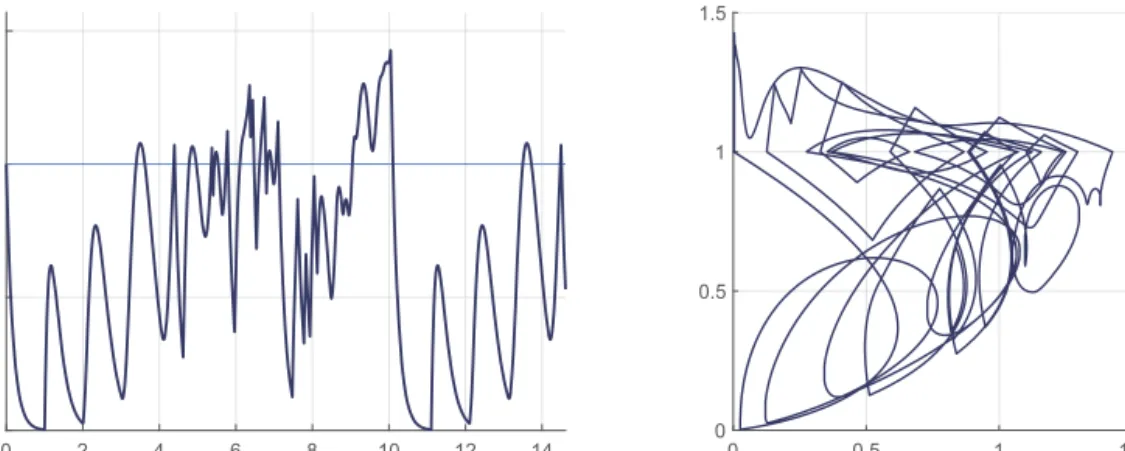
Althoughtheobtainedperiodicorbitsarestable,theirprojectionsRt →(x(t),(x(t−1)))∈R2can becomplicated.
©2021TheAuthor(s).PublishedbyElsevierInc.ThisisanopenaccessarticleundertheCCBY-NC-ND license(http://creativecommons.org/licenses/by-nc-nd/4.0/).
MSC:34K13;34K39;65G30;65Q20
Keywords:Mackey–Glassequation;Limitingnonlinearity;Periodicorbit;Returnmap;Computer–assistedproof
* Correspondingauthor.
E-mailaddress:krisztin@math.u-szeged.hu(T. Krisztin).
https://doi.org/10.1016/j.jde.2021.05.052
0022-0396/©2021TheAuthor(s).PublishedbyElsevierInc.ThisisanopenaccessarticleundertheCCBY-NC-ND license(http://creativecommons.org/licenses/by-nc-nd/4.0/).
1. Introduction
The Mackey–Glass equation
y(t )= −ay(t )+b y(t−τ ) 1+yn(t−τ )
with positive parameters a, b, τ, nwas introduced in 1977 by Michael Mackey and Leon Glass [28] as a model of feedback control of blood cells. This simple-looking differential equation with a single delay attracted the attention of many mathematicians since its hump-shaped nonlinearity causes entirely different dynamics compared to the case where the nonlinearity is monotone. See the work [25] of Lasota for a similar model. There exist several rigorous mathematical results, numerical and experimental studies on the Mackey-Glass equation showing convergence, oscil- lations of solutions, and complicated behavior, see e.g. [1,6,14,16,26,27,35]. Despite the intense research, the dynamics is not fully understood yet.
By rescaling the time we may assume τ=1. Therefore, we consider
y(t )= −ay(t )+bfn(y(t−1)) (En) where a >0, b >0, n ≥4, and fn(ξ ) =ξ /[1 +ξn] for ξ ≥0. The natural phase space to study (En) is C+=C([−1, 0], (0, ∞)), see [8,10]. For each ψ∈C+there is a unique solution yn,ψ: [−1, ∞) →(0, ∞)with yn,ψ(s) =ψ (s), −1 ≤s≤0. The solutions define the continuous semiflow Fn: [0, ∞) ×C+(t, ψ ) →yn,ψt ∈C+, where ytn,ψ(s) =yn,ψ(t+s), −1 ≤s≤0.
If a≥b >0 then it is elementary to show that yψ(t ) →0 as t→ ∞for all ψ∈C+. In the rest of the paper we assume b > a >0. Then there is a global attractor A⊂C+, that is, A⊂C+ is compact and nonempty, Fn(t, A) =Afor all t≥0, and Aattracts all bounded subsets of C+. The unique positive zero ζn0of [0, ∞) ξ → −aξ+bfn(ξ ) ∈Rdefines the unique equilib- rium point ζˆn0∈C+of Fnby ζˆn0(s) =ζn0, −1 ≤s≤0. It is easy to see that, for fixed b > a >0, there exists an N (a, b) ≥4 so that ζˆn0 is unstable for n ≥N (a, b), and, as nincreases, ζˆn0is a source of periodic orbits via local Hopf bifurcations, see e.g. [44]. On the other hand, the papers [15] by Karakostas et al. and [9] by Gopalsamy et al. give conditions for the global attractivity of the unique positive equilibrium of (En) for b > a >0, and nis below a certain constant given in terms of a, b. Our result is valid for some b > a >0 and nis large.
The maximum of fn is at ξn0=1/√n
n−1. Assuming n > b/(b−a), the inequality ξn0< ζn0 follows. Liz, Röst and Wu [26,35] gave conditions to guarantee A⊂ {ψ∈C+:ψ (s) > ξn0}, that is Ais in the region where the feedback is monotone decreasing. This means that the structure of Acan be studied by using the Poincaré–Bendixson type theorem of Mallet-Paret and Sell [31], see also [17,41].
If ξn0< ζn0 (a consequence of n > b/(b−a)) then there is a unique ζn1 ∈(0, ξn0) with bfn(ζn1) =aζn0, and (ξ−ζn0)(−aζn0+bfn(ξ )) <0 for ξ∈(ζn1, ∞) \ {ζn0}. Consequently, if t >0, y(t ) =ζn0and y(t−1) ∈(ζn1, ζn0)then y(t ) >0, and if t >0, y(t ) =ζn0and y(t−1) > ζn0then y(t ) <0. This means a negative feedback condition in the region (ζn1, ∞)with respect to ζn0. Then the inclusion A⊂ {ψ∈C+:ψ (s) > ζn1}(which can be guaranteed by following [26,35]) allows to apply the results obtained for equations with negative feedback resulting in a Morse de- composition of A, see [30,32]. In particular, periodic orbits and some connections between them can be obtained in this way. In addition, under the negative feedback condition complicated dy- namics is possible, see [11,24]. The work of Lani-Wayda [23] shows chaos for an equation with
a hump-shaped nonlinearity, similar to fn, however, the result is not applicable for (En). A major problem in delay differential equations is to prove complicated dynamics for the Mackey–Glass equation (En).
We emphasize that, in general, for equation (En) the global attractor Ais not in a region of C+where the negative feedback condition holds with respect to the positive equilibrium.
The aim of this paper is to construct periodic orbits for equation (En) for some parameter val- ues a, b, n. The obtained periodic orbits are hyperbolic, orbitally stable, exponentially attractive with asymptotic phase. In the proof we use the limiting Mackey–Glass equation
x(t )= −ax(t )+bf (x(t−1)) (E∞)
where f (ξ ) =limn→∞fn(ξ ), that is, f (ξ ) =ξ for ξ ∈ [0, 1), f (1) =1/2, and f (ξ ) =0 for ξ >1. Theorem3.1shows that if the parameters b > a >0 are given so that the hypothesis (H) equation (E∞) has an ω-periodic solution p:R →Rwith the following properties:
(i) p(0) =1, p(t ) >1 for all t∈ [−1, 0), (ii) (p(t ), p(t−1)) =(1, a/b)for all t∈ [0, ω]
holds then there exists an n∗≥4 such that, for all n ≥n∗, equation (En) has a periodic solution pn:R →Rwith period ωn>0 so that the periodic orbits On= {pnt :t∈ [0, ωn]}are hyperbolic, orbitally stable, exponentially attractive with asymptotic phase, and ωn→ω, dist{On,O} →0 as n → ∞, where O= {pt:t∈ [0, ω]}.
In order to get periodic orbits for equation (En) by the application of Theorem3.1, hypothesis (H) needs to be verified. We have two types of results in this direction: analytical and computer- assisted proofs. First, Proposition4.1shows that (H) is satisfied if b is large comparing to a, namely b >max{aea, ea−e−a}. Another result, whose proof can be found in [18], is Propo- sition 4.2 when b is sufficiently close to a. More precisely, for every a >0 there exists an ε0=ε0(a) >0 such that for the parameters a, b with b∈(a, a+ε0)condition (H) holds. If a >0 is fixed and bk→a+as k→ ∞then the minimal period of the obtained periodic solu- tion tends to ∞. The most interesting examples for a, b, such that (H) is valid, are obtained by applying rigorous computer-assisted techniques, see Proposition4.5.
The results of this paper can be summarized as follows.
Theorem 1.1. If the pair of parameters a, bsatisfies either the condition of Proposition4.1, or Proposition4.2, or aand bare given in Proposition4.5, then there exists an n∗=n∗(a, b) ≥4 such that for all n ≥n∗equation (En)has a hyperbolic, orbitally stable, exponentially attractive periodic orbit with asymptotic phase.
The shapes of the obtained periodic solutions (depending on a, b, n) vary from simple looking slowly oscillating solutions (with respect to ζn0) to solutions with complex structures, see the figures at the end of the paper. For some of the periodic solutions xguaranteed by Theorem1.1 the projections R t →(x(t ), x(t−1)) ∈R2produce complicated looking structures, and the figures are similar to those obtained in numerical studies and were believed to be a sign of chaotic dynamics generated by (En)
As the proofs are technical, we give a brief overview of the key steps. A solution of (E∞) is defined as a continuous function x: [−1, t∗) →Rwith 0 < t∗≤ ∞such that the map [0, t∗) t →f (x(t−1)) ∈Ris locally integrable and
x(t )=e−a(t−τ )x(τ )+ t τ
e−a(t−s)f (x(s−1)) ds
holds for all 0 ≤τ < t < t∗. It is easy to see that for any initial function ϕ∈C+ there is a unique solution x=xϕ : [−1, ∞) →(0, ∞)satisfying x0=ϕ. However, comparing solutions with ϕ >1 and ϕ≡1, one sees that there is no continuous dependence on initial data in C+. By choosing
Cr+= {ψ∈C+:ψ−1(c)is finite for allc∈(0,1]}
as a phase space, the solutions of (E∞) define the continuous semiflow [0, ∞) (t, ϕ) →xtϕ∈ Cr+.
If ϕ∈C+r and the solution x=xϕof (E∞) satisfies the additional property (x(t ), x(t−1))=
1,a b
(1.1) for all t in a fixed interval [0, M], then Proposition2.6shows that, for large n, the solution yn,ψ, ψ∈C+, of (En) remains close to xϕ on the interval [0, M]provided they are close on the interval [0, 1]. Condition (1.1) guarantees that, if x(t ) =xϕ(t )is close to 1 and the derivative x(t )exists, then x(t ) = −ax(t ) +bf (x(t−1))is not close to zero, and this makes it possible to show that the measure of the set {t∈ [−1, M−1]: |xϕ(t ) −1| < δ}is bounded by Kδ for a fixed K >0, and for all small δ >0. Therefore, for most of the times t∈ [0, M], one has xϕ(t−1) /∈(1 −δ, 1 +δ), that is, xϕ(t−1)is not close to the discontinuity point of f allowing the application of perturbation type arguments. Another key fact is that, for each δ∈(0, 1), fn(ξ ) →f (ξ )as n → ∞uniformly in ξ∈ [0, 1 −δ]∪ [1 +δ, ∞). This convergence ensures that, for large n, maxt∈[0,1]|xϕ(t ) −yn,ψ(t )| is small provided ϕ(s) ≥1 +δ, ψ (s) ≥1 +δ, s∈ [−1, 0]. See Propositions2.5and 2.6for the precise results.
Hypothesis (H) implies the existence of a small γ >0 so that for a translate q of p one has q0∈Sγ = {ψ∈C+:ψ (s) ≥ψ (0) =1 +γ , s∈ [−1, 0]}. Theorem3.1states that, for large n, the solution curves [0, ∞) t →ytn,ψ∈C+of (En) starting in Sγ return to Sγ, that is, ytn,ψ∈Sγ
for some t >0. A crucial property of the Mackey–Glass nonlinearity is that, for n ≥4, the polynomial bound supξ >0|fn(ξ )|≤n/4 is valid, while for a fixed γ >0, supξ≥1+γ|fn(ξ )|≤ n/[1 +(1 +γ )n]tending to zero exponentially as n → ∞. This guarantees that, for large n, the return map Sγ ψ →ytn,ψ∈Sγ is a contraction, and its fixed point determines a stable periodic orbit of (En).
The paper is organized as follows. Section2 shows the basic properties of the solutions of equation (E∞) in the phase space Cr+. In addition, it gives the technical conditions ensuring that the solutions of (E∞) with certain regularity properties are approximated on compact intervals by the solutions (En) for large n. Section3proves that, for large n, under hypothesis (H) equation (En) has a stable periodic orbit close to the orbit guaranteed by (H). Section4contains analytical and rigorous computer-assisted tools to find parameter values b > a >0 with hypothesis (H).
The paper is concluded by figures demonstrating the variety of the obtained periodic orbits of the Mackey–Glass equation (En).
We remark that a well known and widely applied technique in the study of a delay differential equation of the form y(t ) = −ay(t ) +bgn(y(t−1)), with a parameter n, is to consider the lim- iting equation x(t ) = −ax(t ) +bg(x(t−1))with the assumption that the limiting nonlinearity g(ξ ) =limn→∞gn(ξ )is a step function with finite steps. The idea turned out to be very success- ful to prove a variety of dynamical properties, see the papers [4,11,19–21,34,36,40,42,43,45].
For example, the search for periodic orbits can be reduced to a finite dimensional problem in this way. For an equation with a piece-wise linear limiting nonlinearity g, like f in equation (E∞), the search for periodic orbits is still an infinite dimensional problem. For a delay differential equation, different from (En), Mackey et al. [29] introduced the limiting nonlinearity f as in this paper, and constructed stable periodic orbits for the original equation. The technique of Mackey et al. [29] applies to equation (En) provided bis large comparing to a, and yields a periodic so- lution of (En) with a relatively simple shape. In the present paper the situation of [29] is covered by Proposition4.1(together with Theorem3.1).
Acknowledgment
This research was supported by the National Research, Development and Innovation Fund, Hungary, grants NKFIH-K-129322, NKFIH-1279-2/2020, NKFIH KKP 129877, 2020-2.1.1- ED-2020-00003, by the EU-funded Hungarian Grant EFOP-3.6.2-16-2017-0015, and by the grant TUDFO/47138-1/2019-ITM of the Ministry for Innovation and Technology, Hungary. F.B.
was also supported by the János Bolyai Research Scholarship of the Hungarian Academy of Sciences, and by the grant UNKP-20-5 - New national excellence program of the Ministry for Innovation and Technology from the source of the National Research, Development and Innova- tion Fund.
2. Preliminary results
Let R, C, N, N0denote the set of real numbers, complex numbers, positive integers, nonneg- ative integers, respectively. Let C be the Banach space C([−1, 0], R)equipped with the norm ϕ=maxs∈[−1,0]|ϕ(s)|. For a continuous function u :I→Rdefined on an interval I, and for t, t−1 ∈I, ut∈Cis given by ut(s) =u(t+s), s∈ [−1, 0]. Introduce the subsets
C+= {ψ∈C:ψ (s) >0 for alls∈ [−1,0]}, C+r =
ψ∈C+:ψ−1(c)is finite for allc∈(0,1]
of C where ψ−1(c) = {s∈ [−1, 0] :ψ (s) =c}. C+ and Cr+are metric spaces with the metric d(ϕ, ψ ) = ϕ−ψ. For a finite set Slet #Sdenote the number of elements of the set S.
Let a, b, nbe real positive parameters with b > a >0 and n ≥4. Define the function fn: [0,∞)ξ → ξ
1+ξn∈R, and its limit when n → ∞
f (ξ )= lim
n→∞fn(ξ )= lim
n→∞
ξ 1+ξn =
⎧⎪
⎨
⎪⎩
ξ if 0≤ξ <1
1
2 ifξ=1 0 ifξ >1 Set
ξn0= 1
√n
n−1, ξn1= n n+1
n−1.
Then 0 < ξn0<1 < ξn1, and ξn0, ξn1are the only zeros of fn, fnin (0, ∞), respectively.
Proposition 2.1. Let n ≥4.
(i) For each ε∈(0, 1), fn(ξ ) →f (ξ ), as n → ∞, uniformly in ξ∈ [0, ∞) \(1 −ε, 1 +ε).
(ii) If ξ >0then |fn(ξ )| ≤n/4.
(iii) If ξ >1then |fn(ξ )| ≤n/(1 +ξn).
Proof. (i) If 0 ≤ξ≤1 −εthen
|fn(ξ )−f (ξ )| = ξn+1
1+ξn ≤(1−ε)n+1. If ξ ≥1 +εthen
|fn(ξ )−f (ξ )| =fn(ξ )= 1
1/ξ+ξn−1≤(1+ε)1−n.
(ii) From fn(ξ ) = [1 −(n −1)ξn]/(1 +ξn)2it is easy to see that fn(ξ ) ∈ [0, 1)for ξ ∈(0, ξn0], and fn(ξ ) <0 for ξ > ξn0. From
fn(ξ )=nξn−1[(n−1)ξn−(n+1)] (1+ξn)3
it follows that fnhas a minimum at ξn1. For the minimum value fn(ξn1) = −(n −1)2/(4n) ≥ −n/4 holds. Therefore, −n/4 ≤fn(ξ ) <1 for all ξ >0. This proves (ii).
(iii) If ξ >1 then
|fn(ξ )| =(n−1)ξn−1
(1+ξn)2 <(n−1)ξn
(1+ξn)2 < n−1 1+ξn < n
1+ξn and (iii) holds.
Consider the equations
y(t )= −ay(t )+bfn(y(t−1)) (En) and
x(t )= −ax(t )+bf (x(t−1)). (E∞) A solution of equation (En) on [−1, ∞)with initial function ψ∈C+is a continuous function y: [−1, ∞) →R so that y0=ψ, the restriction y|(0,∞) is differentiable, and equation (En) holds for all t >0. The solutions are easily obtained from the variation-of-constants formula for ordinary differential equations on successive intervals of length one,
y(t )=e−a(t−k)y(k)+b t
k
e−a(t−s)fn(y(s−1)) ds, (2.1)
where k∈N0, k≤t ≤k+1. Hence one can find that each ψ∈C+ uniquely determines a solution y=yn,ψ: [−1, ∞) →Rwith y0n,ψ=ψ, and yn,ψ(t ) >0 for all t≥0. In addition, one sees that yn,ψ satisfies the integral equation
yn,ψ(t )=e−a(t−τyn,ψ(τ )+b t τ
e−a(t−s)f (yn,ψ(s−1)) ds (0≤τ < t <∞). (2.2)
The solutions define the continuous semiflow
Fn: [0,∞)×C+(t, ψ ) →ytn,ψ∈C+.
For equation (E∞) with the discontinuous f, we use formula (2.1) with f instead of fn
to define solutions for (E∞). A solution of equation (E∞) with initial function ϕ∈C+ is a continuous function x=xϕ: [−1, tϕ) →R with some 0 < tϕ≤ ∞such that x0=ϕ, the map [0, tϕ) s →f (x(s−1)) ∈Ris locally integrable, and
x(t )=e−a(t−k)x(k)+b t k
e−a(t−s)f (x(s−1)) ds, (2.3)
holds for all k∈N0and t∈ [0, tϕ)with k≤t≤k+1.
It is not difficult to show that, for any ϕ ∈C+, there is a unique solution xϕ of equation (E∞) on [−1, ∞). However, comparing solutions with initial functions ϕ >1, ϕ≡1, one sees that there is no continuous dependence on initial data in C+. Therefore we restrict our attention to the subset Cr+ of C+. The choice of Cr+ as a phase space guarantees not only continuous dependence on initial data, but also allows to compare certain solutions of equations (E∞) and (En) for large n.
Proposition2.2below shows that, for all ϕ∈Cr+, equation (E∞) has a unique solution xϕ on [−1, ∞)with xtϕ∈Cr+for all t≥0. Once we have the existence of xϕ: [−1, ∞) →R, it is elementary to obtain the integral equation
xϕ(t )=e−a(t−τ )xϕ(τ )+b t τ
e−a(t−s)f (xϕ(s−1)) ds (0≤τ < t <∞). (2.4)
Proposition 2.2. For each ϕ∈Cr+ there is a unique maximal solution xϕ : [−1, ∞) →R of equation (E∞). The maximal solution xϕ satisfies:
(i) xtϕ∈Cr+for all t≥0,
(ii) if t >0and xϕ(t−1) =1, then xϕis differentiable at t, and equation (E∞)holds at t. The map
F: [0,∞)×Cr+(t, ϕ) →xϕt ∈Cr+ is a continuous semiflow.
Proof. Step 1.Let ϕ∈Cr+be given. Then there exists a sequence (sl)Ll=0so that −1 ≤s0< s1<
. . . < sL≤0 and ϕ−1(1) = {s0, . . . , sL}. Set J = {t0, . . . , tL}with tl =sl+1, l∈ {0, . . . , L}. The function [0, 1]s →f (ϕ(s−1)) ∈ [0, 1]is bounded, and continuous at all ξ∈ [0, 1]\J. Consequently, it is integrable on [0, 1]. It follows that the definition
x0=ϕ, x(t )=e−atx(0)+b t 0
e−a(t−s)f (x(s−1)) ds, t∈ [0,1] (2.5)
of x: [−1, 1] →Rgives a continuous function. Moreover, x is differentiable at each point of (0, 1]\J, and equation (E∞) holds for all t∈(0, 1]\J
Step 2.Assume xt∈C+is not satisfied for all t∈ [0, 1]. Then, by x0=ϕ∈C+, there is a minimal t∗∈(0, 1]with x(t∗) =0. As Jis a finite set, there is an ε >0 so that [t∗−ε, t∗) ∩J= ∅, and (E∞) holds for all t∈(t∗−ε, t∗). Clearly,
x(t )= −ax(t )+bf (x(t−1))≥ −ax(t ) for allt∈(t∗−ε, t∗), and it follows that
x(t )≥x(t∗−ε)e−a(t−t∗+ε)≥x(t∗−ε)e−aε for allt∈(t∗−ε, t∗).
Hence, by the continuity of x, we obtain the contradiction x(t∗) >0. Therefore xt ∈C+for all t∈ [0, 1].
Step 3.If xt∈Cr+is not true for all t∈ [0, 1], then there exists a c∈(0, 1]so that {t∈ [0, 1] : x(t ) =c}is an infinite set. As J is finite, we may choose an open interval I⊂(0, 1)so that I∩J= ∅and Ic= {t∈I: x(t ) =c}is infinite. Note that x is differentiable on I, (E∞) holds on I.
By ϕ∈Cr+, one may assume that x(t−1) /∈ {ac/b, 1}for all t∈I. Observe ac/b <1. This fact and the continuity of x0=ϕallow us to distinguish three cases.
Case 1: x(t−1) >1 for all t∈I. Then x(t ) = −ax(t ) <0 for all t∈I, and hence x is strictly decreasing on I, a contradiction to the fact that Icis infinite.
Case 2:x(t−1) < ac/bfor all t∈I. Since Icis infinite, there is a t∗∈I with x(t∗) =cand x(t∗) ≥0. On the other hand, we have
x(t∗)= −ax(t∗)+bf (x(t∗−1))= −ac+bx(t∗−1)) <−ac+bac b =0,
a contradiction.
Case 3:ac/b < x(t−1) <1 for all t∈I. Similarly to Case 2, as Icis infinite, there is t∗∗∈I with x(t∗∗) =cand x(t∗) ≤0. From (E∞) it follows that
x(t∗∗)= −ax(t∗∗)+bf (x(t∗∗−1))= −ac+bx(t∗∗−1) >−ac+bac b =0, a contradiction.
Therefore xt∈Cr+for all t∈ [0, 1].
Step 4.So far we proved that, for any ϕ∈Cr+, (2.5) defines a continuous extension xof ϕto [−1, 1], and xt∈Cr+for all t∈ [0, 1]. This procedure can be repeated to find a unique continuous function x: [−1, ∞) →Rsuch that x0=ϕ, xt ∈C+r for all t≥0, and equation (2.3) holds for all k∈N0and t∈ [k, k+1]. Therefore, a unique solution xϕ exists on [−1, ∞), and statement (i) is satisfied as well. Moreover, according to the remark preceding the proposition, the integral equation (2.4) holds for xϕ.
If xϕ(¯t−1) =1 then xϕ(s−1) =1 for all s∈ [τ, t]provided τ <t < t¯ and τ, t are close to
¯
t. As the only discontinuity of f is at ξ =1, by applying the fundamental theorem of calculus, statement (ii) follows from the integral equation (2.4).
Step 5.Let t1≥0, t2>0, ϕ∈Cr+. We claim that the semigroup property F (t1+t2, ϕ) = F (t2, F (t1, ϕ)) holds. It is sufficient to show the semigroup property for t2∈(0, 1], since the case t2>1 can be obtained from repeated application of the case t2∈(0, 1]. So, let t2∈(0, 1].
Let ψ=F (t1, ϕ) =xtϕ1. We have to show xtψ2 =F (t2, ψ ) =F (t1+t2, ϕ) =xϕt1+t2, that is, xψ(t2+θ ) =xϕ(t1+t2+θ ), θ∈ [−1, 0].
If t2+θ≤0, then xψ(t2+θ ) =ψ (t2+θ ) =xϕ(t1+t2+θ ). If t2+θ >0 then, by (2.4) with τ=0, t=t2+θand ψ=xtϕ1,
xψ(t2+θ )=e−a(t2+θ )ψ (0)+b
t2+θ 0
e−a(t2+θ−s)f (ψ (s−1)) ds. (2.6)
By (2.4) with τ=0, t=t1, one has
ψ (0)=xϕ(t1)=e−at1x(0)+b
t1
0
e−a(t1−s)f (xϕ(s−1)) ds. (2.7)
Substituting (2.7) into (2.6) and using ψ (s−1) =xϕ(t1+s−1), we obtain
xψ(t2+θ )=e−a(t1+t2+θ )x(0)+b
t1+t2+θ 0
e−a(t1+t2+θ−s)f (xϕ(s−1)) ds
=xϕ(t1+t2+θ ).
Therefore, xtψ2 =xtϕ
1+t2.
Step 6.For any fixed ϕ∈Cr+, the continuity of [0, ∞) t →F (t, ϕ) ∈Cr+follows from the uniform continuity of xϕon compact subintervals of [−1, ∞).
Step 7. Now we show that, for each fixed t ≥0, the map Cr+ϕ →F (t, ϕ) ∈Cr+ is con- tinuous. Suppose t ∈ [0, 1]. Let ε > be given, and let ϕm→ϕ in Cr+. The finite set ϕ−1(1) can be covered by open intervals with total length less than ε/(3b). Let U be the union of these open intervals. Clearly, f (ϕm(s)) →f (ϕ(s))uniformly in s∈ [−1, 0]\U as m → ∞.
Thus, there is m0∈Nso that, for all m ≥m0, sups∈[−1,0]\U|f (ϕm(s)) −f (ϕ(s))| < ε/(3b)and ϕm−ϕ < ε/3. Then, from (2.3) we obtain that, for every t∈ [0, 1]and m ≥m0,
F (t, ϕm)−F (t, ϕ) ≤ sup
t∈[−1,1]|xϕm(t )−xϕ(t )|
≤ ϕm−ϕ +b
⎛
⎜⎝
U
+
[−1,0]\U
⎞
⎟⎠|f (ϕm(s))−f (ϕ(s))|ds
<ε 3+b ε
3b +b ε 3b =ε.
Therefore, ϕm→ϕin C+r implies F (t, ϕm) →F (t, ϕ)as m → ∞uniformly in t∈ [0, 1]. This fact combined with the semigroup property gives that, in case ϕm→ϕ in Cr+, F (t, ϕm) → F (t, ϕ)as m → ∞uniformly on tin compact subintervals of [0, ∞).
Step 8. The continuity of F in t from Step 6 and the continuity of F in ϕ uniformly on t in compact subintervals of [0, ∞)from Step 7 together yield the continuity of F jointly in (t, ϕ) ∈ [0, ∞) ×Cr+. This completes the proof.
Next we prove a boundedness property.
Proposition 2.3. Let ϕ∈Cr+, ψ∈C+and n ≥4.
(i) If ϕ and ψ are in C([−1, 0], (0, b/a))then the segments xtϕ and yn,ψt are in C([−1, 0], (0, b/a))for all t≥0. The same holds for C([−1, 0], (0, b/a]).
(ii) There exist t∗(ϕ) ≥0, t∗∗(ψ ) ≥0such that xtϕ∈C([−1, 0], (0, b/a))for all t≥t∗(ϕ), and yn,ψt ∈C([−1, 0], (0, b/a))for all t≥t∗∗(ϕ).
(iii) If yn,ψ(t0) ≤b/a for some t0≥0then |(yn,ψ)(t )| <2bholds for all t > t0. Similarly, if xϕ(t1) ≤b/a for some t1≥0then |(xϕ)(t )| <2b holds for all t > t1for which (xϕ)(t ) exists.
Proof. Let ϕ∈Cr+ and ψ∈C+ be given. Let zdenote either xϕ or yn,ψ. Then, by (2.2) and (2.4), for 0 ≤τ < t <∞, we have
z(t )=e−a(t−τ )z(τ )+b t τ
e−a(t−s)g(z(s−1)) ds
where g=f if z=xϕ, and g=fnif z=yn,ψ.
If z(τ ) ≤b/afor some τ≥0 then, by g≤1, for all t≥τ
z(t )≤ b
ae−a(t−τ )+b t τ
e−a(t−s)ds=b a.
If z(τ ) < b/athen z(t ) < b/afollows for all t > τ. Hence, statement (i) is immediate.
In order to show (ii), by the first part of the proof it suffices to find a t0≥0 with z(t0) < b/a.
Assuming z(t ) ≥b/afor all t≥0, from the integral equation for z, for t >1 one gets
z(t )=e−a(t−1)z(1)+b t
1
e−a(t−s)g(z(s−1)) ds
≤e−a(t−1)z(1)+b a
1−e−a(t−1)
sup
ξ≥b/a
g(ξ ).
Hence, by using b > a >0 and supξ≥b/ag(ξ ) <1, it follows that lim supt→∞z(t ) < b/a, a contradiction. Therefore, (ii) holds.
Statement (iii) is obvious from equations (En), (E∞) and Proposition2.2.
For γ >0 define
γ= {ϕ∈C:ϕ(s)≥1+γ fo alls∈ [−1,0]}.
Clearly, γ ⊂C+. The difference of two solutions of (En) with initial functions from γ can be estimated as follows.
Proposition 2.4. Let γ >0, ψ∈γ, χ∈γ, and n ≥4. Let y=yn,ψ and z=zn,χdenote the solutions of (En)on [−1, ∞)with initial functions ψand χ, respectively. Then, for each integer M≥0, we have
|y(t )−z(t )| ≤
|ψ (0)−χ (0)| + bn
1+(1+γ )nψ−χ 1+bn 4
M
for all t∈ [0, M+1].
Proof. For t∈ [0, 1]from the integral equation (2.1) for yand zwith k=0, by using Proposi- tion2.1,
|y(t )−z(t )| ≤e−at|ψ (0)−χ (0)| +b sup
ξ≥1+γ
|f(ξ )| t 0
e−a(t−s)|y(s−1)−z(s−1)|ds
≤
|ψ (0)−χ (0)| + bn
1+(1+γ )nψ−χ
follows. This means that the statement holds for M=0.
Let = |ψ (0) −χ (0)| +
bn/(1+(1+γ )n)
ψ−χ. Suppose that j ≥1 is an integer and for all t∈ [0, j]the inequality
|y(t )−z(t )| ≤
1+bn 4
j−1
is valid. Then
yj−zj ≤
1+bn 4
j−1
holds as well. Using Proposition2.1and the last inequality, from the integral equations (2.1) for yand zwith t∈ [j, j+1]and k=j, we obtain
|y(t )−z(t )| ≤e−a(t−j )|y(j )−z(j )| +bsup
ξ >0
|f(ξ )| t j
e−a(t−s)|y(s−1)−z(s−1)|ds
≤
1+bn 4
yj−zj
≤
1+bn 4
j
, and the proof is complete.
For ϕ∈Cr+, τ ≥0 and δ∈(0, 1)define
(ϕ, τ, δ)= {t∈(τ, τ+1): |xϕ(t )−1|< δ}.
By the continuity of xϕ, the set (ϕ, τ, δ)is the union of disjoint open intervals. Let |(ϕ, τ, δ)| denote the sum of the lengths of these open intervals.
For ϕ∈Cr+, τ ≥0 and δ0∈(0, min{a/b, 1 −a/b})let
(ϕ, τ, δ0)= {t∈ [τ−1, τ] :xϕ(t )∈ {1, a/b+δ0, a/b−δ0}}. By Proposition2.2, the set (ϕ, τ, δ0)is finite, that is #(ϕ, τ, δ0) <∞.
For δ0∈(0, min{a/b, 1 −a/b})set
Nδ0=[1−δ0,1+δ0]×a b −δ0,a
b +δ0
.
The next result guarantees that the solution xϕof equation (E∞) spends relatively little time in a neighborhood of the discontinuity ξ=1 of f, that is, |(ϕ, τ, δ)|is small.
Proposition 2.5. Let ϕ∈C+r , M≥1, δ0∈(0, min{a/b, 1 −a/b})and γ0∈Nbe given such that xϕ(t ), xϕ(t−1)
∈/Nδ0 for allt∈ [0, M] (2.8)
and
#(ϕ, τ, δ0)≤γ0 for allτ∈ [0, M−1] (2.9) hold. Define K0=2(1 +γ0)/[(b−a)δ0].
Then, for any δ∈(0, δ0],
|(ϕ, τ, δ)| ≤K0δ for allτ ∈ [0, M−1]. (2.10) Proof. Set x=xϕ, and fix τ∈ [0, M−1]and δ∈(0, δ0].
Define the subsets
U= {t∈(τ, τ+1):x(t−1)=1 andx(t−1) /∈ [a/b−δ0, a/b+δ0]}, V = {t∈(τ, τ+1):x(t−1)∈ [a/b−δ0, a/b+δ0]},
W= {t∈(τ, τ+1):x(t−1)=1}
of (τ, τ+1). Clearly, U, V , Ware disjoint, and (τ, τ+1) =U∪V∪W. Setting
=(ϕ, τ, δ)= {t∈(τ, τ+1): |x(t )−1|< δ}, we have
=∩(τ, τ+1)=(∩U )∪(∩V )∪(∩W ).
Observe ∩V = ∅by (2.8), and Wis finite by Proposition2.2, and ∩Uis an open subset of (τ, τ+1). It follows that || = | ∩U|.
By (2.9) the set =(ϕ, τ, δ0)is a finite subset of [τ, τ+1]. Therefore the open set U can be written as
U= N j=1
(αj, βj)
where
τ ≤α1< β1≤α2< β2≤. . .≤αN< βN≤τ+1.
The set =(ϕ, τ, δ0)contains the points β1, α2, β2, . . . , αN−1, βN−1, αN, and possibly more points. Since βj=αj+1can happen for j∈ {1, . . . , N−1}, the set contains at least N−1 points. Thus,
N≤1+#≤1+γ0. Clearly
∩U= N j=1
∩(αj, βj) .
For a given (αj, βj)there are three cases according to whether x(t−1) >1, or a/b+δ0<
x(t−1) <1, or 0 < x(t−1) < a/b−δ0 for all t∈(αj, βj). In all cases, x(t )exists and equation (E∞) holds for all t∈(αj, βj)since x(t−1) =1.
Case 1: x(t−1) >1 for all t ∈(αj, βj). If t ∈ ∩(αj, βj)then x(t ) >1 −δ, and, by δ0< a/b,
x(t )= −ax(t )≤ −a(1−δ)≤ −a(1−δ0) <−(b−a)δ0.
Case 2:a/b+δ0< x(t−1) <1 for all t∈(αj, βj). If t∈ ∩(αj, βj)then x(t ) <1 +δ, and, by δ0< a/b,
x(t )= −ax(t )+bx(t−1) >−a(1+δ)+b(a/b+δ0) > (b−a)δ0.
Case 3:0 < x(t−1) < a/b−δ0for all t∈(αj, βj). If t∈ ∩(αj, βj)then x(t ) >1 −δ, and, by δ0< a/b,
x(t )= −ax(t )+bx(t−1) <−a(1−δ)+b(a/b−δ0) <−(b−a)δ0. CLAIM.Either ∩(αj, βj) = ∅, or ∩(αj, βj) =
αj,βj
for some αj, βjwith αj≤αj<
βj≤βj.
Proof of the Claim. Suppose ∩(αj, βj) = ∅. Since ∩(αj, βj)is open, it suffices to show that for all t1, t2, t3in (αj, βj)with t1< t2< t3and t1∈, t3∈we have t2∈.
Assume t2∈/. Then either x(t2) ≥1 +δ, or x(t2) ≤1 −δ. If x(t2) ≥1 +δthen, by t1, t3∈, t2∈(t1, t3)and continuity, there exist t2∗∈(t1, t2]and t2∗∗∈ [t2, t3)so that
x(t2∗)=x(t2∗∗)=1+δ, x(t ) <1+δ for allt∈(t1, t2∗)∪(t2∗∗, t3).
On the other hand, in Cases 1, 2, 3 we obtain
x(t2∗) <0, x(t2∗∗) >0, x(t2∗) <0,
respectively, which is a contradiction. The possibility x(t2) ≤1 −δ similarly leads to a contra- diction. Therefore, t2∈, and the Claim holds.
According to the above Claim, assume ∩(αj, βj) = αj,βj
with αj ≤αj <βj ≤βj. Then one of the Cases 1–3 holds for all t∈(αj, βj), and
|x(t )| ≥(b−a)δ0 for allt∈(αj,βj).
In particular, x(t )does not change sign in (αj, βj). Observe that (αj, βj) ⊂implies |x(βj) − x(αj)| ≤2δ. Combining the above facts we obtain
2δ≥ |x(βj)−x(αj)| = |
βj
αj
x(t ) dt| =
βj
αj
|x(t )|dt≥(b−a)δ0(βj−αj).
Hence
|∩(αj, βj)| =βj−αj≤ 2δ (b−a)δ0. Since j∈ {1, . . . , N}was arbitrary,
|| = |∩U| = N j=1
|∩(αj, βj)| ≤N 2δ
(b−a)δ0≤2(1+γ0)
(b−a)δ0δ=K0δ, and the proof is complete.
By Proposition2.1, for each δ∈(0, 1)there exists n1=n1(δ) ≥4 so that
|fn(ξ )−f (ξ )|< δprovidedn≥n1(δ), ξ≥0, and|ξ−1| ≥δ.
Now we are able to guarantee that, for large n, the solutions of equation (En) remain close to a solution of equation (E∞) on a compact interval, provided they are close on the interval [0, 1].
Proposition 2.6. Let ϕ∈Cr+, an integer M >1, δ0∈(0, min{a/b, 1 −a/b})and γ0∈N be given so that conditions (2.8)and (2.9)are satisfied. Let
K0= 2
(b−a)δ0(1+γ0), B=1+2b(K0+1)andδ1=δ0 2B−M.
Then for all δ∈(0, δ1], for all n ≥n1(δ), and for all ψ∈C+, for the solutions x=xϕ of (E∞) and y=yn,ψof (En),
y1−x1< δ implies |y(t )−x(t )|< δBM (t∈ [0, M+1]).
Proof. Let δ∈(0, δ1], n ≥n1(δ), and ψ∈C+be fixed. Set x=xϕ and y=yn,ψ. Suppose that
y1−x1< δ.
It is sufficient to show that
yj+1−xj+1< δBj for allj∈ {0, . . . , M}. We prove by induction. Assume that j∈ {1, . . . , M}is given, and
yj−xj< δBj−1.