Periodic solutions with long period for the Mackey–Glass equation
Dedicated to Professor Jeffrey R. L. Webb on the occasion of his 75th birthday
Tibor Krisztin
BBolyai Institute, University of Szeged, Aradi vértanúk tere 1, Szeged, H–6720, Hungary Received 8 November 2020, appeared 21 December 2020
Communicated by Gennaro Infante
Abstract. The limiting version of the Mackey–Glass delay differential equationx0(t) =
−ax(t) +b f(x(t−1)) is considered where a,b are positive reals, and f(ξ) = ξ for ξ ∈ [0, 1), f(1) = 1/2, and f(ξ) = 0 for ξ > 1. For every a > 0 we prove the existence of an ε0 = ε0(a) > 0 so that for all b ∈ (a,a+ε0) there exists a periodic solution p = p(a,b) :R →(0,∞)with minimal period ω(a,b) such thatω(a,b)→ ∞ as b → a+. A consequence is that, for each a > 0, b ∈ (a,a+ε0(a)) and sufficiently largen, the classical Mackey–Glass equationy0(t) =−ay(t) +by(t−1)/[1+yn(t−1)]
has an orbitally asymptotically stable periodic orbit, as well, close to the periodic orbit of the limiting equation.
Keywords: Mackey–Glass equation, periodic solution, limiting nonlinearity, discontin- uous right-hand side, long period.
2020 Mathematics Subject Classification: 34K13, 34K39, 34K06.
1 Introduction
The Mackey–Glass equation
y0(t) =−ay(t) +b y(t−τ) 1+yn(t−τ)
with positive parameters a,b,τ,n was proposed to model blood production and destruction in the study of oscillation and chaos in physiological control systems by Mackey and Glass [13]. This simple-looking differential equation with a single delay attracted the attention of many mathematicians since its hump-shaped nonlinearity causes entirely different dynamics compared to the case where the nonlinearity is monotone. See [16] for a similar equation.
There exist several rigorous mathematical results, numerical and experimental studies on the Mackey–Glass equation showing convergence of the solutions, oscillations with different
BEmail: krisztin@math.u-szeged.hu
characteristics, and the complexity of the dynamics, see e.g. [1,3,6,7,9,15,17–19,22,23]. Despite the intense research, the dynamics is not fully understood yet.
The recent paper [2] studies the classical Mackey–Glass delay differential equation
y0(t) =−ay(t) +b fn(y(t−1)) (En) wherea,b,nare positive reals, fn(ξ) =ξ/[1+ξn]forξ ≥0,τ=1 can be assumed by rescaling the time. [2] constructs stable periodic solutions of (En) for someb> a >0 and large n. The periodic solutions can have complicated shapes, see [2]. A limiting version of (En) plays a key role in the construction. The function f(ξ) =limn→∞ fn(ξ)is given by f(ξ) =ξ forξ ∈ [0, 1),
f(1) =1/2, and f(ξ) =0 forξ >1. The equation
x0(t) =−ax(t) +b f(x(t−1)) (E∞) is called the limiting Mackey–Glass equation.
Let R, C and N denote the set of real numbers, complex numbers and positive inte- gers, respectively. Let C be the Banach space C([−1, 0],R) equipped with the norm kϕk = maxs∈[−1,0]|ϕ(s)|. For a continuous function u : I → R defined on an interval I, and for t,t−1∈ I,ut ∈Cis given byut(s) =u(t+s),s∈[−1, 0]. Introduce the subsets
C+={ψ∈C:ψ(s)>0 for alls∈ [−1, 0]}, Cr+=nψ∈C+ :ψ−1(c)is finite for allc∈ (0, 1]o
of Cwhere ψ−1(c) = {s ∈ [−1, 0]: ψ(s) = c}. C+ and Cr+ are metric spaces with the metric d(ϕ,ψ) =kϕ−ψk.
A solution of equation (En) on[−1,∞)with initial functionψ∈C+is a continuous function y:[−1,∞)→Rso thaty0=ψ, the restrictiony|(0,∞)is differentiable, and equation (En) holds for all t > 0. The solutions are easily obtained from the variation-of-constants formula for ordinary differential equations on successive intervals of length one,
y(t) =e−a(t−k)y(k) +b Z t
k e−a(t−s)fn(y(s−1))ds (1.1) where k ∈ N∪ {0}, k ≤ t ≤ k+1. Hence it is well known that each ψ ∈ C+ uniquely determines a solutiony=yn,ψ :[−1,∞)→Rwith yn,ψ0 =ψ, andyn,ψ(t)>0 for allt ≥0.
For equation (E∞) with the discontinuous f, we use formula (1.1) with f instead of fn to define solutions. A solution of equation (E∞) with initial function ϕ ∈ C+ is a continuous functionx =xϕ :[−1,tϕ)→Rwith some 0<tϕ≤∞such that x0= ϕ, the map[0,tϕ)3s7→
f(x(s−1))∈Ris locally integrable, and x(t) =e−a(t−k)x(k) +b
Z t
k e−a(t−s)f(x(s−1))ds (1.2) holds for allk∈N∪ {0}andt∈ [0,tϕ)withk≤ t≤k+1.
It is easy to show that, for any ϕ ∈ C+, there is a unique solution xϕ of equation (E∞) on [−1,∞). However, comparing solutions with initial functions ϕ> 1, ϕ≡ 1, one sees that there is no continuous dependence on initial data inC+. Therefore we restrict our attention to the subsetCr+ of C+. The choice of C+r as a phase space guarantees not only continuous dependence on initial data, but also allows to compare certain solutions of equations (E∞) and (En) for largen. This is not used here, but it is important in [2]. [2] proves that for eachϕ∈C+r
there is a unique maximal solution xϕ :[−1,∞)→Rof equation (E∞). The maximal solution xϕ satisfiesxϕt ∈ Cr+ for allt ≥0; and ift >0 andxϕ(t−1)6=1, then xϕ is differentiable att, and equation (E∞) holds att.
One of the main results of [2] is as follows.
Theorem 1.1. If the parameters b> a>0are given so that
(H) equation(E∞)has anω-periodic solution p:R→Rwith the following properties:
(i) p(0) =1, p(t)>1for all t ∈[−1, 0), (ii) (p(t),p(t−1))6= (1,a/b)for all t∈ [0,ω]
holds then there exists an n∗ ≥ 4 such that, for all n ≥ n∗, equation (En) has a periodic solution pn:R→Rwith periodωn>0so that the periodic orbits
On={pnt :t ∈[0,ωn]}
are hyperbolic, orbitally stable, exponentially attractive with asymptotic phase, moreover, ωn → ω, dist{On,O} →0as n→∞, whereO= {pt :t∈[0,ω]}.
[2] shows that in case bis large comparing to a, namely b > max{aea,ea−e−a}, then (H) is satisfied. In addition, by using a rigorous computer-assisted technique, [2] gives parameter values a,bsuch that (H) is valid, and the obtained stable periodic orbits for the Mackey–Glass equation may have complicated structures.
[2] remarks that (H) holds if b > a > 0 andb is sufficiently close to a, and refers to this work for the proof. The aim of this paper is to prove this fact, namely the following result.
Theorem 1.2. For every a> 0there exists anε0 = ε0(a)>0 such that for the parameters a,b with b∈(a,a+ε0)condition (H) holds.
In particular, for the periodic solution p= p(a,b)of equation(E∞)the minimal periodω =ω(a,b) satisfiesω >5, and there exists aσ=σ(a,b)∈(4,ω−1)so that
0< p(t)<1for all t∈(0,σ); p(t)>1for all t∈ (σ,ω).
Moreover, if a >0is fixed and(bk)∞k=1is a sequence in(a,a+ε0(a)),limk→∞bk =a thenσ(a,bk)→
∞,ω(a,bk)→∞as k→∞.
Theorems1.1 and1.2immediately imply the following result for equation (En).
Theorem 1.3. For each a>0there exists anε0= ε0(a)>0such that for every b∈(a,a+ε0)there exists an n∗ =n∗(a,b)≥4so that, for all n≥ n∗, equation(En)has a periodic solution pn:R→R with minimal period ωn(a,b)so that the periodic orbits
On={pnt :t ∈[0,ωn]}
are hyperbolic, orbitally stable, exponentially attractive with asymptotic phase. Moreover, if (bk)∞k=1 is a sequence in(a,a+ε0(a))withlimk→∞bk =a, nk >n∗(a,bk)thenωn(a,bk)→∞as k→∞.
Note that the papers [8] by Karakostas et al. and [5] by Gopalsamy et al. give conditions for the global attractivity of the unique positive equilibrium of (En) for b > a > 0, and n is below a certain constant given in terms of a,b. Theorem1.3requiresnto be large.
Section 2 contains the proof of Theorem 1.2. The proof requires the study of a special solution of a linear autonomous delay differential equation. If ϕ ∈ Cr+ is any function such
that ϕ(s) >1 for s ∈ [−1, 0)and ϕ(0) =1 then the unique solution x = xϕ of equation (E∞) satisfies x(t) = e−at for t ∈ [0, 1]. In order to find a periodic solution of (E∞) as stated in Theorem1.2 we consider the linear autonomous equation
u0(t) =−au(t) +bu(t−1)
for t > 1 withu(t) = e−at, t ∈ [0, 1]. If we find a T > 0 such that u(t) < 1 for t ∈ (0,T), u(T) = 1, u(t) > 1 for t ∈ (T,T+1], then it is straightforward to see that x(t) = u(t) for all t ∈ [0,T+1]. Then, equation (E∞) gives x0(t) = −ax(t) for all t > T+1 as long as x(t−1)> 1. Hence there exists anω > T+1 withx(ω) = 1 andx(t)> 1 for allt ∈ (T,ω). By the fact f(ξ) = 0 for ξ > 1, the solution x does not change on [0,∞) if ϕ is replaced by xω, and consequentlyx(t) =x(t+ω)follows for allt ≥ −1. Therefore the proof of Theorem 1.2is reduced to the existence of a T > 0 withu(t)< 1 fort ∈ (0,T), u(T) =1, u(t)> 1 for t∈ (T,T+1]. Property (H)(ii) is guaranteed byu0(T)>0.
We remark that the use of a limiting equation in order to study nonlinear delay differential equations when the nonlinearity is close to its limiting function is not new. We refer to the papers [10–12,21,24–26] where the limiting step function reduces the search of periodic solutions to a finite dimensional problem. The limiting Mackey–Glass nonlinearity f is not a step function. The introduction of the limiting Mackey–Glass equation does not reduce the search for periodic solutions to a finite dimensional problem, nevertheless it can simplify it. The paper [14] considered the limiting Mackey–Glass nonlinearity to construct periodic solutions for an equation different from (En). The result of [14] is analogous to the case when bis large comparing toa, mentioned above for the Mackey–Glass equation.
2 The proof of Theorem 1.2
The proof is divided into eight steps. The desired periodic solution of equation (E∞) will be anω-periodic extension of a functionw:[0,ω]→R. We constructwin the remaining part of this section.
Step 1.Let a>0 be fixed, and consider the characteristic function h:C×R3(z,ε)7→z+a−(a+ε)e−z ∈C
of the linear delay differential equation v0(t) = −av(t) + (a+ε)v(t−1). By h(0, 0) = 0, D1h(0, 0) = 1+a, and D2h(0, 0) = −1, the Implicit Function Theorem can be applied to get that there areε1 ∈(0, min{a, 1/4}),r1 ∈ (0, 1)and aC1-smooth mapλ0 : (−ε1,ε1)→Csuch that λ0(0) = 0, h(λ0(ε),ε) = 0, and (λ0(ε),ε) is the unique solution of h(z,ε) = 0 in the set {z ∈ C : |z| < r1} ×(−ε1,ε1). Since a and ε are real in the equation h(z,ε) = 0, (z,ε) is a solution together with(z,ε). Then, by uniqueness, it follows thatλ0(ε)∈R, ε∈(−ε1,ε1).
Chapter XI of [4] applies to get that the zeros of the characteristic function h(z,ε) for ε∈(−ε1,ε1)are λ0(ε)∈Rand a sequence of pairs λj(ε),λj(ε)∞
j=1with λ0(ε)>Reλ1(ε)>Reλ2(ε)>· · ·>Reλj(ε)→ −∞ as j→∞ and
Imλj∈ (2j−1)π, 2jπ
(j∈N).
Ifε=0 thenλ0(0) =0, and consequently Reλ1(0)<0. Fix c∈(0,a)so that Reλ1(0)<−2c.
Notice that the choice ofcdepends only ona.
Differentiating the equationh(λ0(ε),ε) =0 with respect toε we obtainλ00(0) =1/(1+a), and thus
λ0(ε) = ε
1+a +η(ε)
with a function η : (−ε1,ε1) → R satisfying limε→0η(ε)/ε = 0. Applying the above repre- sentation for λ0(ε), we assume (in addition to the above properties of ε1) that ε1 is so small that
λ0(ε)< 2ε
1+2a for all ε∈(0,ε1), (2.1) where the equality 2ε/(1+2a) =ε/(1+a) +ε/[(1+a)(1+2a)]shows that this is possible.
By Rouché’s theorem [20] there exists anε2∈ (0,ε1)such that Reλ1(ε)< −2c for allε∈[0,ε2]. In particular,h(z,ε)6=0 on the line{−c+is: s∈R}for all ε∈[0,ε2].
Step 2. Forε∈ (0,ε2)consider the unique solutionv:[−1,∞)→Rof the linear equation v0(t) =−av(t) + (a+ε)v(t−1) (t >0) (2.2) with initial function v0(s) = e−a(s+1), −1 ≤ s ≤ 0. Remark that v and λ0 depend on ε as well. Taking the Laplace transform of both sides of (2.2) and expressing the Laplace transform L(v)(z)ofv,
L(v)(z) = 1 h(z,ε)
"
e−a+ (a+ε)1−e−(z+a) z+a
#
is obtained where the right hand side can be written asF(z,ε) =F1(z) +F2(z,ε)with F1(z) = e
−a
z+a, F2(z,ε) = a+ε (z+a)h(z,ε).
According to Chapter I of [4], by taking the inverse Laplace transform, function v can be written as
v(t) =eλ0tResλ0F(z,ε) + 1
2πe−ct lim
T→∞ Z T
−TeistF(−c+is,ε)ds (t >0).
As F1(z)is holomorphic in a neighborhood of λ0, one finds Resλ0F(z,ε) = Resλ0F2(z,ε). By using that h(z,ε)has a simple zero atλ0, andλ0+a= (a+ε)e−λ0, we get
Resλ0F(z,ε) = a+ε
(λ0+a)D1h(λ0,ε) = a+ε
(λ0+a)(1+ (a+ε)e−λ0) = e
λ0
1+a+λ0. Fort ≥1, integration by parts leads to
Z T
−T
eistF1(−c+is)ds= eist
it
e−a a−c+is
s=T s=−T
+
Z T
−T
eist it
ie−a
(a−c+is)2 ds.
Thus
Tlim→∞ Z T
−TeistF1(−c+is)ds
≤
Z ∞
−∞
eist it
ie−a (a−c+is)2
ds≤K1
with
K1 =2 Z ∞
0
e−a
(a−c)2+s2ds.
Let s0 = 2(a+1)ec. The continuous function (s,ε) 7→ h(−c+is,ε) ∈ C is nonzero on the set [−s0,s0]×[0,ε2]. So there exists k > 0 such that |F2(−c+is,ε)| ≤ k on the compact set [−s0,s0]×[0,ε2]. If|s| ≥s0,ε∈[0,ε2]then, by the choice ofs0,
|h(−c+is,ε)| ≥ |a−c+is| − |(a+ε)ec−is| ≥(a−c)2+s21/2
−(a+1)ec
≥ 1 2
(a−c)2+s21/2
. Consequently
lim
T→∞ Z T
−TeistF2(−c+is,ε)ds
≤
Z ∞
−∞|F2(−c+is,ε)|ds
≤2 Z s0
0 k ds+2 Z ∞
s0
a+1
(1/2)[(a−c)2+s2]ds
=K2 with
K2 =2ks0+4 Z ∞
s0
(a+1) (a−c)2+s2ds.
Notice that bothK1 andK2 are independent ofε∈ (0,ε2). Summarizing the above estimations we obtain that
v(t) = e
λ0(t+1)
1+a+λ0
+rˆ(t) (t ≥1) for some continuous function ˆr :[1,∞)→Rsatisfying
|rˆ(t)| ≤Keˆ −ct (t≥1)
with ˆK= (K1+K2)/(2π). Note that ˆr depends onε, however ˆK andcare independent ofε.
Step 3. For ε ∈ (0,ε2) define the function u : [0,∞) → R by u(t) = v(t−1), t ≥ 0. Then u(t) =e−atfort∈ [0, 1],uis differentiable on(1,∞)and satisfies
u0(t) =−au(t) + (a+ε)u(t−1) (t>1). (2.3) Moreover, definingr(t) =rˆ(t−1)fort≥2,K= Keˆ c,uhas the representation
u(t) = e
λ0t
1+a+λ0+r(t) (t≥2) (2.4) with the continuous functionr :[2,∞)→Rsatisfying
|r(t)| ≤Ke−ct (t ≥2). (2.5)
From equation (2.3)
u(t) =e−a(t−1)u(1) +
Z t
1
(a+ε)e−a(t−s)e−a(s−1)ds
=e−at[1+ (a+ε)ea(t−1)] (t ∈[1, 2])
and
u0(t) =e−at[−a−a(a+ε)ea(t−1) + (a+ε)ea] (t∈(1, 2]). Define
t0= t0(ε) =1+1
a − 1
(a+ε)ea. Chooseε3 ∈(0,ε2]so that
ε3< a
1−a e−a−1+a provided a∈ (0, 1), and letε3= ε2if a≥1.
Supposeε∈(0,ε3). Thent0 =t0(ε)∈(1, 2)is the unique zero ofu0 in(1, 2), and it is easy to see that
tmax∈[1,2]u(t) =u(t0) =e−at0[1+ (a+ε)ea(t0−1)] = a+ε a exp
ae−a a+ε −1
. (2.6)
Step 4. In this step we show the following CLAIM:
(i) For each k∈N
t∈[kmax+1,k+2]u(t)≤1+ ε a
t∈[maxk,k+1]u(t), and
(ii) for each N ∈N
t∈[Nmax+1,N+2]u(t)≤1+ ε a
N
tmax∈[1,2]u(t).
Let k ∈ N be given. If maxt∈[k+1,k+2] ≤ maxt∈[k,k+1]u(t) then the stated inequality obvi- ously holds fork. If maxt∈[k+1,k+2]u(t)>maxt∈[k,k+1]u(t), then there exists at1∈(k+1,k+2] such that u0(t1) ≥ 0 andu(t1) = maxt∈[k+1,k+2]u(t). Equation (2.3) at t = t1 and u0(t1) ≥ 0 imply the inequality −au(t1) + (a+ε)u(t1−1)≥0. Hence
t∈[kmax+1,k+2]u(t) =u(t1)≤ a+ε
a u(t1−1)≤ 1+ ε a
t∈[maxk,k+1]u(t), that is, the stated inequality is satisfied. This proves (i).
A repeated application of (i) gives (ii):
max
t∈[N+1,N+2]u(t)≤1+ ε a
max
t∈[N,N+1]u(t)≤1+ ε a
2
max
t∈[N−1,N]u(t)
≤ · · · ≤1+ ε a
N
tmax∈[1,2]u(t). Step 5. Chooseξ0∈(exp(e−a−1), 1). The function
(0,∞)3ε7→ a+ε a exp
ae−a a+ε−1
∈R
strictly increases and its limit is exp(e−a−1)asε →0+. Therefore there exists an ε4∈ (0,ε3) such that
a+ε a exp
ae−a a+ε −1
< ξ0
for allε∈(0,ε4).
By the equality (2.6) in Step 3 and the choice of ε4, for all ε ∈ (0,ε4), the inequality maxt∈[1,2]u(t)<ξ0holds. Then by the CLAIM in Step 4
t∈[max1,N+2]u(t)<1+ ε a
N
ξ0 (2.7)
follows for allN∈ N.
For a given N∈N, from (2.7) one gets
t∈[max1,N+2]u(t)<1 providedε∈(0,ε4)is so small that
ε< ah
(1/ξ0)1/N−1i
. (2.8)
Step 6.Let N∈N\ {1, 2}be given. We look for a condition onε ∈(0,ε4)to guarantee u0(t)>0 for all t> N. (2.9) Equation (2.3) gives that
au(t)<(a+ε)u(t−1) for allt >N (2.10) is sufficient to yield (2.9). By the representation (2.4) condition (2.10) is equivalent to
a
1+a+λ0eλ0th 1+ ε
a
e−λ0−1i
> ar(t)−(a+ε)r(t−1) (t> N),
that is
1+ ε a
e−λ0 −1> 1+a+λ0
a e−λ0t[ar(t)−(a+ε)r(t−1)] (t > N). Fromε<1, 0< λ0(ε)<1 and (2.5) one obtains
1+a+λ0
a e−λ0t[ar(t)−(a+ε)r(t−1)]
< (a+2)(2a+1)
a Ke−c(t−1)
< (a+2)(2a+1)
a Kece−cN (t > N). Recall that, by the choice ofε1in Step 1,
λ0(ε)< 2ε 2a+1. Hence
e−λ0(ε)>1−λ0(ε)>1− 2ε 2a+1. Thus, by usingε1 <1/4 as well,
1+ ε
a
e−λ0(ε)−1> 1+ ε a
1− 2ε 2a+1
−1
= ε−2ε2
a(2a+1) > ε 2a(2a+1).
Consequently, (2.9) holds if, in addition toε ∈(0,ε4),
ε>ξ1e−cN (2.11)
with ξ1=2(a+2)(2a+1)2Kec.
Step 7.In order to satisfy conditions (2.8) and (2.11) simultaneously considera
(1/ξ0)1/N−1 andξ1e−cN. By L’Hospital’s rule
Nlim→∞
ξ1e−cN
a[(1/ξ0)1/N−1] =0.
Therefore there exists an integer N0>2 such that ξ1e−cN
a
(1/ξ0)1/(N+1)−1 <1 for all integersN ≥N0. (2.12) Defineε∗ ∈(0,ε4)so that
ε∗ <ah
(1/ξ0)1/N0 −1i . Let ε ∈ (0,ε∗)be fixed. By ε < ε∗ and limN→∞a
(1/ξ0)1/N−1
= 0 there exists a maximal integer N(ε)≥ N0 so that
ε <ah
(1/ξ0)1/N(ε)−1i
. (2.13)
The maximality of N(ε)≥ N0 and inequality (2.12) imply ξ1e−cN(ε)< ah
(1/ξ0)1/(N(ε)+1)−1i
≤ε.
Therefore, we arrive at the inequality
ξ1e−cN(ε)<ε< ah
(1/ξ0)1/N(ε)−1i
, (2.14)
that is, for everyε ∈(0,ε∗)inequalities (2.11) and (2.8) hold with N= N(ε).
Step 8. By Steps 5–7, for eachε ∈ (0,ε∗)there exists an integer N = N(ε)> 2 such that the unique continuous function u = u(ε) : [0,∞) → R satisfying u(t) = e−at for t ∈ [0, 1], and equation (2.3) on(1,∞)has the properties
1=u(0)>u(t)>0 for all t∈(0,N+2), u0(t)>0 for all t> N,
u(t)→∞ ast →∞.
(2.15)
The last property is clear from λ0(ε)>0, (2.4) and (2.5).
From (2.15) it follows that there exits a unique σ(ε) > N(ε) +2 > 4 so that u(σ(ε)) = 1 andu0(σ(ε))> 0. Fromu0(σ(ε))> 0 it is clear thatu(σ(ε)−1)6= a/(a+ε). The maximality of N(ε)in inequality (2.13) implies thatN(ε)→∞,σ(ε)→∞asε→0+.
Letω(ε) =σ(ε) +1+ (1/a)logu(σ(ε) +1)>5. Define the functionw:[0,ω(ε)]→Rby w(t) =
(u(t) ift∈ [0,σ(ε) +1], u(σ(ε) +1)e−a(t−σ(ε)−1) ift∈ [σ(ε) +1,ω(ε)].
Thenw(t)>1 for allt ∈(σ,ω), andw(ω) =1. Let p:R→Rbe theω(ε)-periodic extension ofwtoR.
For the fixeda >0 setε0= ε∗. Observe thatc,K, and consequentlyξ0,ξ1, depend only on a. Then relation (2.12) shows thatN0 is also a function ofa. Therefore,ε0 depends only ona.
Ifb∈(a,a+ε0)then the above constructed p(ε)withε= b−a ∈(0,ε∗)is clearly anω(ε)- periodic solution of equation (E∞) satisfying (H). Setting ω(a,b) = ω(ε) andσ(a,b) = σ(ε), we see that all statements of Theorem1.2are satisfied, and the proof is complete.
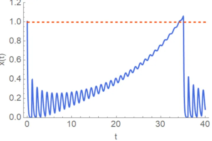
The typical shape of the periodic solutions obtained in this paper for (E∞) is shown in Figure2.1 witha=9, b=9.7.
Figure 2.1: The periodic solution of (E∞) fora=9, b=9.7
Acknowledgements
This research was supported by the grants NKFIH-K-129322, NKFIH-1279-2/2020 of the Min- istry for Innovation and Technology, Hungary, and by the EU-funded Hungarian Grant EFOP- 3.6.2-16-2017-0015.
The author thanks the reviewer for the relevant comments that contributed to improving the paper.
References
[1] P. Amil, C. Cabeza, A. C. Marti, Exact discrete-time implementation of the Mackey–
Glass delayed model, IEEE Transactions on Circuits and Systems II: Express Briefs62(2015), 681–685.https://doi.org/10.1109/TCSII.2015.2415651
[2] F. Á. Bartha, T. Krisztin, A. Vígh, Stable periodic orbits for the Mackey–Glass equation, preprint.
[3] J. B. van den Berg, C. Groothedde, J.-P. Lessard, A general method for computer- assisted proofs of periodic solutions in delay differential problems,J. Dynam. Differential Equations(2020).https://doi.org/10.1007/s10884-020-09908-6
[4] O. Diekmann, S. A. van Gils, S. M. Verduyn Lunel, H.-O. Walther, Delay equa- tions. Functional, complex, and nonlinear analysis, Applied Mathematical Sciences, Vol.
110, Springer-Verlag, New York, 1995. https://doi.org/10.1007/978-1-4612-4206-2;
MR1345150
[5] K. Gopalsamy, S. I. Trofimchuk, N. R. Bantsur, A note on global attractivity in models of hematopoiesis,Ukraïn. Mat. Zh.50(1998), 5–12; reprinted inUkrainian Math. J.50(1998), 3–12.https://doi.org/10.1007/BF02514684;MR1669243
[6] U. an der Heiden, H.-O. Walther, Existence of chaos in control systems with de- layed feedback, J. Differential Equations 47(1983), 273–295. https://doi.org/10.1016/
0022-0396(83)90037-2;MR688106
[7] L. Junges, J. A. C. Gallas, Intricate routes to chaos in the Mackey–Glass delayed feed- back system,Phys. Lett. A376(2012), 2109–2116.https://doi.org/10.1016/j.physleta.
2012.05.022
[8] G. Karakostas, Ch. G. Philos, Y. G. Sficas, Stable steady state of some population models, J. Dynam. Differential Equations 4(1992), 161–190. https://doi.org/10.1007/
BF01048159;MR1150401
[9] G. Kiss, G. Röst, Controlling Mackey–Glass chaos,Chaos27(2017), 114321.https://doi.
org/10.1063/1.5006922;MR3716183
[10] T. Krisztin, M. Polner, G. Vas, Periodic solutions and hydra effect for delay differential equations with nonincreasing feedback,Qual. Theory Dyn. Syst.16(2017), 269–292.https:
//doi.org/10.1007/s12346-016-0191-2;MR3671725
[11] T. Krisztin, G. Vas, Large-amplitude periodic solutions for differential equations with delayed monotone positive feedback, J. Dynam. Differential Equations 23(2011), 727–790.
https://doi.org/10.1007/s10884-011-9225-2;MR2859940
[12] T. Krisztin, G. Vas, The unstable set of a periodic orbit for delayed positive feed- back, J. Dynam. Differential Equations 28(2016), 805–855. https://doi.org/10.1007/
s10884-014-9375-0;MR3537356
[13] M. C. Mackey, L. Glass, Oscillation and chaos in physiological control systems, Science 197(1977), 278–289.https://doi.org/10.1126/science.267326
[14] M. C. Mackey, C. Ou, L. Pujo-Menjouet, J. Wu, Periodic oscillations of blood cell population in chronic myelogenous leukemia, SIAM J. Math. Anal. 38(2006), 166–187.
https://doi.org/10.1137/04061578X;MR2217313
[15] B. Lani-Wayda, Erratic solutions of simple delay equations, Trans. Am. Math. Soc.
351(1999), 901–945.https://doi.org/10.1090/S0002-9947-99-02351-X;MR1615995 [16] A. Lasota, Ergodic problems in biology,Astérisque50(1977), 239–250.MR0490015
[17] E. Liz, G. Röst, Dichotomy results for delay differential equations with negative Schwarzian derivative, Nonlinear Anal. Real World Appl. 11(2010), 1422–1430. https:
//doi.org/10.1016/j.nonrwa.2009.02.030;MR2646558
[18] E. Liz, E. Trofimchuk, S. Trofimchuk, Mackey–Glass type delay differential equations near the boundary of absolute stability, J. Math. Anal. Appl. 275(2002), 747–760. https:
//doi.org/10.1016/S0022-247X(02)00416-X;MR1943777
[19] G. Röst, J. Wu, Domain-decomposition method for the global dynamics of delay differ- ential equations with unimodal feedback, Proc. R. Soc. Lond. Ser. A Math. Phys. Eng. Sci.
463(2007), 2655–2669.https://doi.org/10.1098/rspa.2007.1890;MR2352875
[20] W. Rudin, Real and complex analysis, McGraw-Hill Book Co., New York–Toronto, Ont.- London, 1966.MR0210528
[21] A. L. Skubachevskii, H.-O. Walther, On the Floquet multipliers of periodic solutions to non-linear functional differential equations, J. Dynam. Differential Equations 18(2006), 257–355.https://doi.org/10.1007/s10884-006-9006-5;MR2229980
[22] R. Szczelina, A computer assisted proof of multiple periodic orbits in some first order non-linear delay differential equations,Electron. J. Qual. Theory Differ. Equ. 2016, No. 83, 1–19.https://doi.org/10.14232/ejqtde.2016.1.83;MR3547459
[23] R. Szczelina, P. Zgliczynski, Algorithm for rigorous integration of delay differen- tial equations and the computer-assisted proof of periodic orbits in the Mackey–
Glass equation, Found. Comput. Math. 18(2018), 1299–1332. https://doi.org/10.1007/
s10208-017-9369-5;MR3875841
[24] G. Vas, Configurations of periodic orbits for equations with delayed positive feedback, J. Differential Equations262(2017), 1850–1896.https://doi.org/10.1016/j.jde.2016.10.
031;MR3582215
[25] H.-O. Walther, Contracting return maps for some delay differential equations, in:
T. Faria, P. Freitas (eds.), Topics in functional differential and difference equations (Lisbon, 1999), Fields Inst. Commun., Vol. 29, Amer. Math. Soc., Providence, RI, 2001, pp. 349–
360.MR1821790
[26] H.-O. Walther, Contracting return maps for monotone delayed feedback, Dis- crete Contin. Dyn. Syst. 7(2001), 259–274. https://doi.org/10.3934/dcds.2001.7.259;
MR1808399