A differential equation with a state-dependent queueing delay

A differential equation with a state-dependent queueing delay

Istv´ an Bal´ azs

, Tibor Krisztin

Abstract

We consider a differential equation with a state-dependent delay motivated by a queueing process. The time delay is determined by an algebraic equation involving the length of the queue for which a discontinuous differential equation holds. The new type of state-dependent delay raises some problems that are studied in this paper. We formulate an appropriate framework to handle the system, and show that the solutions define a Lipschitz continuous semiflow in the phase space. The second main result guarantees the existence of slowly oscillating periodic solutions.

Keywords: state-dependent delay, queueing delay, differential inclusion, return map, slow oscillation, fixed point, ejectivity

AMS subject classifications: 34K05, 34K09, 34K13, 34K32

1 Introduction

We consider a system which is composed of a delay differential equation and auxiliary equations defining the delay. The delay differential equation satisfies a negative feedback condition analogously to earlier works by Mallet-Paret and Nussbaum [20, 21], Arino, Hadeler, Hbid and Magal [2, 19], Krisztin and Arino [14], Walther [31, 33, 30, 29]. In [20, 29] the state-dependent delay was an explicitly given function (i.e., no auxiliary equation).

Walther [31, 30] studied problems where the state-dependent delay was defined by an algebraic relation, and in a suitable phase space it was possible to eliminate this auxiliary equation. Arino, Hadeler, Hbid, Magal [2, 19] and Hu, Wu [11] considered an equation where the auxiliary equation for the delay was given by an ordinary differential equation.

Here we study a differential equation with a state-dependent delay where the delay is defined by two auxiliary equations: an algebraic equation and a differential equation with a discontinuous right hand side. The considered system is interesting from the theoretical point of view since previous results do not seem applicable here. On the other hand, the system is a prototype of rate control problems with delays appearing naturally in queueing processes.

The particular model, that motivated our study, was introduced by Ranjan, La and Abed in [26, 25]. The problem is specified for a simple computer network, however,

∗MTA-SZTE Analysis and Stochastics Research Group, Bolyai Institute, University of Szeged, Szeged, Aradi v. tere 1, 6720, Hungary.

†Bolyai Institute, University of Szeged, Szeged, Aradi v. tere 1, 6720, Hungary.

analogous models appear, e.g., in more general computer networks, in road networks, in biological networks, or in general in those processes where a bottleneck phenomenon slows down the performance or capacity of a system, see, e.g., [27, 5, 8]. The model is a fluid model, although data are usually discrete. When we talk about data transfer, we can think of a liquid flowing in a pipe. In the derivation of the model sometimes it is helpful to use a discrete version of the phenomenon and to mention units of data. In these cases the continuous model equations are obtained by taking limits. We hope this does not cause confusion. So, consider a network containing a single user and a single server. The user’s transmission rate satisfies the bound 0 < a ≤ x(t) ≤ b, where b is a user-specific physical limitation, and the lower bound a is due to the fact that the user needs to probe the congestion level of the network by continuously transmitting data. The server processes the incoming data by the capacity c ∈ (a, b). Kelly [12] introduced the utility U(x) and the price p(x) per unit flow of the processing, when the rate isx. Under natural conditions on the functions U(·) and p(·), there is an optimal rate x_∗ ∈ (a, c) (balancing between the utility and the price of processing) as the unique maximum of the expression U(x)−Rx

0 p(y)dy subject to the constraint 0< x≤c, see Kelly et al. [13]. In addition, [13] proposed an end user rate control algorithm as the differential equation

˙

x(t) = κ

x(t)U⁰(x(t))−x(t)p(x(t))

(1.1) where xU⁰(x) is the price per unit time the user is willing to pay for the processing, xp(x) is the price charged by the server, κ > 0 is a gain parameter. The solutions of equation (1.1) converge monotonically to x∗ ast→ ∞. On the other hand, nonmonotone convergence and nonconvergent oscillation around x_∗ arise in some rate control problems.

Equation (1.1) neglects the feedback delays appearing naturally in the system.

The rate control model of Ranjan, La and Abed [26, 25] takes the feedback delays into account. As the rate x(t) can be larger than the capacity of the server, the data arriving at the server may form a single waiting line (a queue) before processing. Let y(t) denote the length of the queue at time t. Suppose that it is bounded from above by q >0, and the units of data reaching the queue with length q are lost. Then, assuming that the transmission time from the user to the server is r₀ ≥ 0, it is natural that for the length y(t) of the queue the differential equation

˙ y(t) =







x(t−r₀)−c if 0< y(t)< q, [x(t−r₀)−c]⁺ if y(t) = 0,

−[x(t−r₀)−c]⁻ if y(t) = q

(1.2)

is satisfied. Here, equation (1.2) is required to hold almost everywhere, and u⁺ = max{u,0},u⁻ = max{−u,0} denote the positive and negative parts of u, respectively.

Suppose that a unit of data, whose processing was completed and the user received an acknowledgement about it at time t, arrived at the queue τ(t) time earlier, i.e., at time t−τ(t), and found a queue with length y(t−τ(t)). As the capacity of the server is c, the given unit of data spent waiting time z(t) = (1/c)y(t−τ(t)) in the queue before its processing started. Let r1 denote the sum of the processing time and the transmission time from the server to the user. Then τ(t) = z(t) +r₁, and this gives the algebraic equation

z(t) = 1

cy(t−z(t)−r1) (1.3)

between y and z.

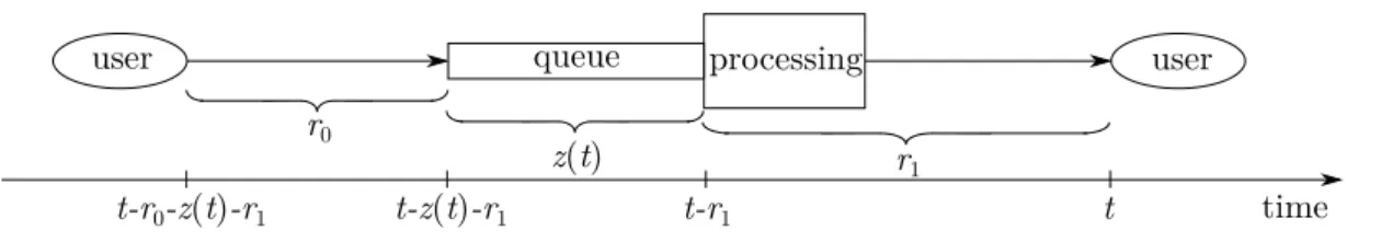
With the waiting time z(t) and the transmission delays r₀, r₁, the user at time t receives an acknowledgement from the server about the processing of that unit of data which was sent at time t−r₀−z(t)−r₁. The server determines a price for a unit rate when it arrives at the server, i.e., at time t−z(t)−r₁. When the processing of a unit ends, the server sends a signal to the user including the identification of the processed unit and the price information p(x(t−z(t)−r₁)). Then the user is able to estimate the price for the rate of data sent att−r₀−z(t)−r₁ asx(t−r₀−z(t)−r₁)p(x(t−z(t)−r₁)).

This led Ranjan, La and Abed [26, 25] to the rate control equation

˙

x(t) =κ

x(t)U⁰(x(t))−x(t−r₀−z(t)−r₁)p(x(t−z(t)−r₁))

(1.4) with a gain parameter κ >0. See figure 1. For similar models we refer to [1, 3].

processing

user queue user

server

time t

t-r₁ t-z(t)-r₁

t-r₀-z(t)-r₁ r₀

z(t) r₁

Figure 1: The process in time.

In this paper we consider rate control equations (like (1.4)) with delay, where the delay is determined by two auxiliary equations, by (1.3) and (1.2), or only by (1.2).

The primary aim of this paper is to find a suitable framework to study the above types of rate control systems. We define a phase space where the corresponding initial value problem has a unique maximal solution. The solutions define a continuous semiflow, and the solution operators are Lipschitz continuous. We believe that this approach can be extended to handle a wide class of systems modeling networks with queueing delays.

Observe that neither the classical results for equations with constant delay [7, 9] nor the recently developed results for equations with state-dependent delay [10, 29] are applicable here.

The papers of Ranjan et al. [17, 15, 16, 23, 24, 25, 26] and [1, 3] consider similar systems, starting from discrete ones, through ordinary and delay differential equations with constant or state-dependent delays, to general network systems. They examine these models from the engineering point of view, comparing the different rate control schemes, like the TCP (transmission control protocol) and its modifications. In these papers, they prove local and global stability of equilibria, show bifurcations, and plot numerical solutions related to their results. However, as far as we know, they do not study the problem of existence, uniqueness, continuous dependence with a mathematical rigor.

The secondary aim is to apply the developed framework, and to show that the rate control defined by System (1.4), (1.2), (1.3) may lead to a slowly oscillating periodic rate around the optimal rate x∗, provided that the stationary solution x=x∗,y = 0, z = 0 is unstable andr₀ = 0. This answers affirmatively a conjecture of Ranjan and his coauthors [24, 22].

Before giving an overview on the main steps toward the results, some notation is introduced. N denotes the set of positive integers, R and C stand for the set of real and complex numbers, respectively. For n ∈N,Rⁿ is then-dimensional Euclidean space with norm | · |. For a closed and bounded interval I let C_I denote the Banach space C(I,R)

equipped with the normkϕk_I = maxs∈I|ϕ(s)|. For Banach spacesE, F with norms k · kE, k · k_F, the norm on E × F is k(u, v)k=kuk_E+kvk_F, u∈ E,v ∈ F.

Set r =r₀ +r₁ +q/c > 0 as an upper bound for the delays. If I ⊆ R is an interval, u : I → R is continuous, r > 0, t and t−r are in I, then u_t ∈ C[−r,0] is defined by u_t(s) =u(t+s), s∈[−r,0].

For a Lipschitz continuous ϕ:I →R, defined on the interval I, let lip(ϕ) = sup

s∈I, t∈I, s<t

ϕ(t)−ϕ(s) t−s

∈[0,∞) and slope(ϕ) =

ϕ(t)−ϕ(s)

t−s : s∈I, t ∈I, s6=t

⊆R.

First we consider a slightly more general system than (1.4), (1.2), (1.3), that is, in the equation we allow more general dependence on the length of the queue than that of (1.4), (1.2), (1.3), and equation (1.3) may or may not hold. Consider the equation

˙

x(t) =F(x_t, y_t) (1.5)

together with (1.2) in the phase spaceX×Y whereX, Y andF are defined as follows. An upper bound K >0 for the absolute value of the right hand side of equation (1.5) comes from the nature of the problem. Then, by x(t)∈[a, b] and the bound K, the subset

X =

ϕ∈C[−r,0]

ϕ([−r,0]) ⊆[a, b], lip(ϕ)≤K

of C[−r,0] will contain all possible segments x_t. Analogously, by y(t) ∈[0, q], x(t) ∈[a, b]

and equation (1.2), for the segments yt, it is natural to introduce the subset Y =

ψ ∈C[−r,0]

ψ([−r,0]) ⊆[0, q], slope(ψ)⊆[a−c, b−c]

of C_[−r,0]. On X ⊂ C_[−r,0], Y ⊂ C_[−r,0], X ×Y ⊂ C_[−r,0]×C_[−r,0] we use the induced subspace topologies and the corresponding norms. By the Arzel`a–Ascoli theorem, X, Y and X×Y are compact subsets of C[−r,0] and C[−r,0]×C[−r,0], respectively. Assume that the map F :X×Y →R has the following properties:

(F1) there exists an L >0 such that, for all ϕ¹, ϕ² ∈X,ψ¹, ψ² ∈Y, F(ϕ¹, ψ¹)−F(ϕ², ψ²)

≤L

ϕ¹−ϕ²

_[−r,0]+

ψ¹−ψ² _[−r,0]

; (F2) max(ϕ,ψ)∈X×Y |F(ϕ, ψ)| ≤K;

(F3) there exists r₂ ∈ (0, r₁] such that F(ϕ, ψ¹) = F(ϕ, ψ²) provided ϕ ∈ X, ψ¹ ∈ Y, ψ² ∈Y, and ψ¹|_[−r,−r2] =ψ²|_[−r,−r2];

(F4) F(ϕ, ψ) > 0 if ϕ ∈ X, ψ ∈ Y, ϕ(0) = a, and F(ϕ, ψ) < 0 if ϕ ∈ X, ψ ∈ Y and ϕ(0) = b.

A solution of System (1.5), (1.2)in the phase spaceX×Y on [−r, ω),ω ≤ ∞, with initial condition x₀ =ϕ∈X, y₀ =ψ ∈Y is a pair of functions

x=x^ϕ,ψ : [−r, ω)→R and y=y^ϕ,ψ : [−r, ω)→R such that

(i) x_t∈X for all t∈[0, ω), x₀ =ϕ;

(ii) x is differentiable on (0, ω);

(iii) y_t ∈Y for all t∈[0, ω), y₀ =ψ;

(iv) equation (1.5) holds on (0, ω);

(v) equation (1.2) holds almost everywhere in (0, ω).

The solution (x, y) = (x^ϕ,ψ, y^ϕ,ψ) on [−r, ω) is called maximal if any other solution (bx,by) with xb0 =ϕ, yb0 =ψ is a restriction of (x, y).

In section 3 we show that, under hypotheses (F1)–(F4), for each (ϕ, ψ) ∈ X × Y, system (1.5), (1.2) has a unique maximal solution x^ϕ,ψ, y^ϕ,ψ

: [−r,∞) → R². The solutions define the continuous semiflow

Φ : [0,∞)×X×Y 3(t, ϕ, ψ)7→

x^ϕ,ψ_t , y^ϕ,ψ_t

∈X×Y,

and, for each t ≥ 0, the solution operators Φ(t,·,·) : X ×Y → X × Y are Lipschitz continuous (theorem 3.4). In order to sketch the main steps of the proof, let (ϕ, ψ)∈X×Y be given. As, by (F3), the value of F(ϕ, ψ) does not depend on ψ

[−r2,0], a standard contraction argument yields T ∈ (0, r₂] and a unique x : [−r, T] → R so that equation (1.5) holds on (0, T), for arbitrary extension of y0 = ψ to y : [−r, T] → R. Next we redefine y : [−r, T] → R on (0, T] such that y_t ∈ Y for all t ∈ [0, T], and equation (1.2) holds almost everywhere on [0, T] with x : [−r, T] → R obtained in the first step. In order to appropriately redefine y: [−r, T]→R on [0, T], we extend the right hand side of (1.2) to an upper semicontinuous multivalued map, and apply a standard result from [6]

for differential inclusions. These two steps combined give a unique solution (x^ϕ,ψ, y^ϕ,ψ) on [−r, T]. By the method of steps the solution can be uniquely extended to a maximal solution on some [−r, ω). Global existence, i.e., ω=∞, follows from (F4).

In order to see that System (1.4), (1.2), (1.3) is a particular case of System (1.5), (1.2) introduce Z = [0, q/c] ⊂ R as a state space for the variable z(t). A crucial fact is the existence of a unique Lipschitz continuous map (lemma 3.5) σ : Y → Z, with Lipschitz constant 1/a, such that

σ(ψ) = 1

cψ(−σ(ψ)−r1) (ψ ∈Y).

Then, for a solution (x, y) : [−r,∞)→R²of System (1.5), (1.2) in the phase space X×Y, defining z(t) =σ(y_t),t≥0, equation (1.3) is always satisfied for all t≥0.

Define a map G:X×Z →R such that

(G1) there exists an L_G >0 such that, for all ϕ¹, ϕ² ∈X,ζ¹, ζ² ∈Z, G(ϕ¹, ζ¹)−G(ϕ², ζ²)

≤L_G

ϕ¹−ϕ²

[−r,0]+

ζ¹−ζ²

; (G2) max(ϕ,ζ)∈X×Z|G(ϕ, ζ)| ≤K;

(G3) G(ϕ, ζ) > 0 if ϕ ∈ X, ζ ∈ Z, ϕ(0) = a, and G(ϕ, ζ) < 0 if ϕ ∈ X, ζ ∈ Z and ϕ(0) =b

hold. If we define F by

F :X×Y 3(ϕ, ψ)7→G(ϕ, σ(ψ))∈R,

then it is straightforward to check that hypotheses (F1)–(F4) are satisfied providedL_G ≤ Lmin{1, a}. In this case System (1.5), (1.2) is equivalent to the system composed of the equations

˙

x(t) =G(x_t, z(t)), (1.6)

(1.2) and (1.3). Then, in the phase space X×Y, for each (ϕ, ψ)∈X×Y, System (1.6), (1.2), (1.3) has the unique solutionx^ϕ,ψ[−r,∞)→R,y^ϕ,ψ : [−r,∞)→R,z^ϕ,ψ : [0,∞)→ Rwhere x^ϕ,ψ, y^ϕ,ψ

is the solution of System (1.5), (1.2) with the above choice ofF, and z^ϕ,ψ(t) =σ(y_t^ϕ,ψ), t≥0.

Defining the map G as G:X×Z 3(ϕ, ζ)7→κ

ϕ(0)U⁰(ϕ(0))−ϕ(−ζ−r0−r1)p(ϕ(−ζ−r1))

∈R, (1.7) System (1.4), (1.2), (1.3) will be a particular case of System (1.6), (1.2), (1.3), see section 5.

In section 3 we show that System (1.6), (1.2), (1.3) can be studied not only in the phase space X ×Y, but also in X × Z with a different notion of solution. For given (ϕ, ζ)∈X×Z, the pair of functions x: [−r,∞)→R,z : [0,∞)→R is called a solution of System (1.6), (1.2), (1.3) in the phase spaceX×Z ifxt ∈X andz(t)∈Z for allt≥0, x₀ =ϕ, z(0) =ζ, x is differentiable and equation (1.6) holds on (0,∞), moreover, there exists a function y : [−r,∞) → R with y_t ∈ Y, z(t) = σ(y_t) for all t ≥ 0, and equation (1.2) is satisfied almost everywhere on [−ζ−r1,∞).

The key technical result (see section 3) to show that System (1.6), (1.2), (1.3) is well posed in X ×Z is that there is a unique Lipschitz continuous map γ : X ×Z → Y so that ψ =γ(ϕ, ζ) satisfies ψ(s) = cζ for s ∈[−r,−ζ −r1], and equation (1.2) holds with x(t) = ϕ(t), y(t) = ψ(t) a.e. in [−ζ−r₁,0]. In particular, ζ = (1/c)ψ(−ζ −r₁). This means that the past of the length of the queue (that isψ ∈Y) can be recovered from the past of the rate (that is ϕ∈X) and from the present waiting time (that is ζ ∈Z). The maps

h:X×Z 3(ϕ, ζ)7→(ϕ, γ(ϕ, ζ))∈X×Y, k:X×Y 3(ϕ, ψ)7→(ϕ, σ(ψ))∈X×Z are Lipschitz continuous, h is injective, andk◦h = id_X×Z, h◦k

_h(X×Z) = id_h(X×Z). Then (see theorem 3.10), for each (ϕ, ζ)∈X×Z, there exists a unique solutionx^ϕ,ζ : [−r,∞)→ R, z^ϕ,ζ : [0,∞)→R of System (1.6), (1.2), (1.3) in the phase space X×Z satisfying the initial condition x^ϕ,ζ₀ =ϕ, z^ϕ,ζ(0) =ζ. Moreover,

Ψ : [0,∞)×X×Z 3(t, ϕ, ζ)7→

x^ϕ,ζ_t , z^ϕ,ζ(t)

∈X×Z

is a continuous semiflow on X×Z, and Ψ(t, ϕ, ζ) =k(Φ(t, h(ϕ, ζ))) for allt ≥0.

In the second part of the paper we study a particular system including the model of Ranjan et al. [26, 25], and show that the optimal equilibrium may be unstable, and in

that case a slowly oscillatory periodic solution appears. Namely, we consider the system

˙

v(t) =−f(v(t))−g(v(t−z(t)−1)) (1.8)

˙ y(t) =







v(t)−d if 0< y(t)< q [v(t)−d]⁺ if y(t) = 0

−[v(t)−d]⁻ if y(t) =q

(1.9)

z(t) = 1

cy(t−z(t)−1) (1.10)

with reals c, q as before, and A < 0 < d < B, and nonlinearities f, g in C¹([A, B],R) satisfying 0 ≤ f(ξ)/ξ ≤ f₁, 0 < g(ξ)/ξ ≤ g₁ for all ξ ∈ [A, B]\ {0} for some f₁ ≥ 0, g₁ >0.

Assume r0 = 0, r1 = 1 in equation (1.4). Condition r0 = 0 guarantees a single delay in equation (1.4), r₁ = 1 can be achieved by rescaling the time. Then, under natural conditions on U, p in equation (1.4), the rate control System (1.4), (1.2), (1.3) will be a particular case of System (1.8), (1.9), (1.10), see Sections 4–5.

Under suitable conditions on f, g, see section 4, proposition 4.1 shows that System (1.8), (1.9), (1.10) is well posed in the phase space X ×Z where

X =

ϕ∈C[−r,0]

ϕ([−r,0])⊆[A, B], lip(ϕ)≤K1 , and r = 1 +q/c,K₀ = (f₁+g₁) max{−A, B}, K₁ =rK₀.

A solution (v, z) of System (1.8), (1.9), (1.10) is calledslowly oscillatoryif for any two zeros t1, t2 ofv with t1 < t2 the inequalityz(t2) + 1< t2−t1 holds. This means that the distance between consecutive zeros of v is larger than the delay.

Inspired by [20] and [19], introduce W =n

(ϕ, ζ)∈ X ×Z ϕ

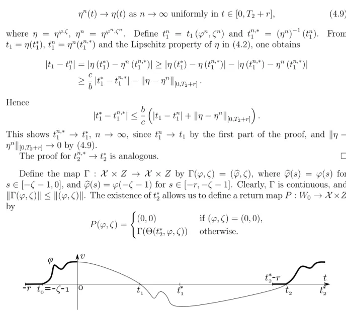
_{[−r,−ζ−1]} ≡0, s7→ϕ(s)e^f1s is nondecreasing, ϕ(0)>0o and W₀ =W ∪ {(0,0)}. Then, for each (ϕ, ζ)∈W, the solutionv =v^ϕ,ζ : [−r,∞)→R, z = z^ϕ,ζ : [0,∞) → R is slowly oscillatory with an infinite number of zeros of v. The second zero t₂ of v in (0,∞) determines t^∗₂ > t₂ so that t₂ = t^∗₂−z(t^∗₂)−1, and a return map P : W₀ → W₀ can be defined by P(0,0) = (0,0), and P(ϕ, ζ) = Γ(Θ(t^∗₂, ϕ, ζ)) for (ϕ, ζ) ∈ W where Γ : X ×Z → X ×Z is given by Γ(ϕ, ζ) = (ϕ, ζ), withb ϕ(s) =b ϕ(s) for s ∈ [−ζ −1,0], and ϕ(s) =b ϕ(−ζ −1) for s ∈ [−r,−ζ −1]. A nontrivial fixed point of P corresponds to a slowly oscillating periodic solution. A classical tool, that we apply here as well, is Browder’s non-ejective fixed point theorem. A large part of section 4 is devoted to the construction of a suitable subset of X ×Z where Browder’s theorem is applicable. We remark that, although the papers [20, 21, 2, 19, 31, 33, 30, 29] consider a similar approach to get slowly oscillating periodic solutions, none of them can be directly applied here, because of the particular definition of the state-dependent queueing delay.

Some steps of the proof are analogous, and other parts require new ideas.

It is a crucial result that P(ϕ, ζ) cannot decay too fast: there are constants θ > 0, ρ > 0 with v^ϕ,ζ(t^∗₂) ≥ θ(ϕ(0))^ρ for all (ϕ, ζ) ∈ W. This fact allows to construct a C²- function α on [0, q/c] such that α(0) = 0, α⁰ > 0, α⁰⁰ > 0 on (0, q/c], α(q/c) is small enough, and the delayed inequality

α

ξ− d c

≥θ(α(ξ))^ρ

ξ ∈

d c,q

c

holds, provided d < q. Defining the compact subsets W_α,K1 =

(ϕ, ζ)∈W₀

ϕ(0) ≥α(ζ) , W_α,K0 =

(ϕ, ζ)∈W_α,K1

lip(ϕ)≤K₀ (1.11)

of X ×Z, the inclusion P(W_α,K1) ⊆ W_α,K0 is satisfied. However, W_α,K1 and W_α,K0 are not convex. Following [19], the subset

V_α,K1 =n

(ψ, ζ)∈C_[−1,0]×Z

ψ([−1,0]) ⊆[0, B], lip(ψ)≤K₁,

[−1,0]3s7→ψ(s)e^f1rs ∈R is nondecreasing, ψ(−1) = 0, ψ(0) ≥α(ζ)

o (1.12) of C[−1,0]×R is compact and convex. The set V_α,K1 can be mapped into W_α,K1 by the streching map Qgiven by Q(ψ, ζ) = (ϕ, ζ) withϕ(s) =ψ(s/(ζ+ 1)), s∈[−ζ−1,0], and ϕ

_{[−r,−ζ−1]} ≡0. The squeezing mapR, defined byR(ϕ, ζ) = (ψ, ζ) withψ(s) =ϕ((ζ+1)s), s ∈[−1,0], maps W_α,K0 into V_α,K1. Browder’s theorem can be applied for the map

Π :V_α,K1 ∈(ψ, ζ)7→R◦P ◦Q(ψ, ζ)∈V_α,K1

to find a non-ejective fixed point of Π in Vα,K1. This yields a non-ejective fixed point of P in W_α,K1 as well. The non-ejective fixed point is nontrivial provided (0,0) ∈ W_α,K1 is ejective. Ejectivity of (0,0) ∈ W_α,K1 follows in a standard way from that of the zero solution of the constant delay equation ˙v(t) =−f(v(t))−g(v(t−1)).

Finally, section 5 gives examples.

2 Preliminary results

In order to study the queue equation (1.2) we recall a basic result of [6] for differential inclusions.

LetJ = [t₀, t₁]⊂ R for some fixed t₀, t₁ ∈R, t₀ < t₁, and let D ⊆R^j be closed. The multivalued map

F : J×D → 2^Rj\ {∅}=

A ⊆R^j, A6=∅

is called upper semicontinuous if F⁻¹(A) is closed in J ×D whenever A ⊆ R^j is closed.

Note that the definition of the inverse image F⁻¹(A) =

(t, y)∈J ×D

F(t, y)∩A6=∅ (2.1)

is different from that of a single valued map.

Letρ(y, D) = infz∈D|y−z| for y∈R^j. For y∈D define T_D(y) =

z ∈R^j : lim inf

λ→0⁺

1

λρ(y+λz, D) = 0

. The following existence result is Theorem 5.1 in [6]:

Theorem A. Suppose that the multivalued map F :J×D→2^Rj\ {∅}is upper semicon- tinuous, for all (t, y)∈J×D the set F(t, y) is closed and convex in R^j,

F(t, y)∩T_D(y)6=∅ for all (t, y)∈J×D,

moreover, there is a Lebesgue integrable c:J →[0,∞) such that, for all (t, y)∈J×D, sup{|z|: z ∈F(t, y)} ≤c(t)(1 +|y|)

holds. Then, for each y₀ ∈ D, there exists an absolutely continuous y :J →D such that y(t₀) =y₀ and the inclusion y(t)˙ ∈F(t, y(t)) holds a.e. on [t₀, t₁].

Assume that E is a Banach space, C ⊂ E is compact and convex in E, the map F : C → C is continuous. A fixed point x₀ ∈ C of F is said to be ejective if there exists an open neighborhood U of x₀ inC such that for eachx∈ U \ {x₀}there exists a positive integer k(x) such that for the iterate F^k(x)(x) ∈ C \ U holds. In section 4 we will apply the following result of Browder [4] on the existence of a non-ejective fixed point.

Theorem B. Assume thatE is a Banach space, C ⊂ E is an infinite dimensional compact and convex subset of E, the map F : C → C is continuous. Then F has a non-ejective fixed point.

For the application of the above result, we have to guarantee the ejectivity of the trivial fixed point of a return map. The proof of the ejectivity uses properties of the linear autonomous equation with constant delay

˙

w(t) =−µw(t)−νw(t−1) (2.2)

where µ ≥ 0 and ν > 0. We recall some basic results from [7, 9, 32]. It is well known that every ϕ ∈ C[−1,0] uniquely determines a solution w^ϕ : [−1,∞) → R of equation (2.2) with w^ϕ|_[−1,0] = ϕ, and the solutions define the strongly continuous semigroup (T(t))t≥0 on [0,∞) ×C[−1,0]. The spectrum of the generator consists of the solutions λ ∈ C of the characteristic equation λ+ µ+νe^−λ = 0. Assume ν > e^−µ−1. Then all points in the spectrum form a sequence of complex conjugate pairs (λ_j, λ_j)^∞_j=1 with Reλ_j >Reλ_j+1,Imλ_j ∈((2j−2)π,(2j−1)π) for allj ∈N, and Reλ_j → −∞asj → ∞.

An explicit criterion for Reλ₁ >0 is ν > ϑ

sinϑ where ϑ∈(0, π) is the unique solution of µ=−ϑcotϑ. (2.3) LetL and Qdenote the realified generalized eigenspaces of the generator associated with the spectral sets {λ₁, λ₁} and {λ_k, λ_k : k ≥ 2}, respectively. Then C[−1,0] = L ⊕ Q. A basis of L is given by the restrictions of the functions

t7→e^Reλ1tsin(Imλ₁t), t7→e^Reλ1tcos(Imλ₁t) to the interval [−1,0].

Let S ⊂ C[−1,0]\ {0} be the set of functions with at most one sign change in [−1,0].

The set S is invariant, i.e., T(t)S⊆S for all t ≥0. Moreover, S∩ Q=∅.

Proposition 2.1. If µ≥0 andν > 0are given such that Reλ₁ >0, i.e., inequality (2.3) holds, and ϕ∈S, then the solution w^ϕ of equation (2.2) is unbounded on [−1,∞).

Proof. Let ϕ ∈ S and w = w^ϕ. From C[−1,0] = L ⊕ Q, S∩ Q = ∅ and ϕ6= 0 it follows that ϕ = ϕ^L +ϕ^Q with ϕ^L ∈ L \ {0}, ϕ^Q ∈ Q. Then w = wL+wQ where wL = w^ϕL and wQ =w^ϕQ. Asϕ^L ∈ L \ {0}, there exist k₁, k₂ ∈ R with k₁²+k²₂ 6= 0 so that, for all t ≥ −1,

wL(t) =e^Reλ1t[k₁sin(Imλ₁t) +k₂cos(Imλ₁t)].

The estimate on the complementary space Q (see, e.g., [7] or [9]) implies that there are δ >0 and M > 0 such that, for allt≥ −1,

|wQ(t)| ≤M e^{(Reλ1−δ)t}. Then, by Reλ₁ >0, it easly follows that w is unbounded.

3 The solution semiflow

Assume that r₀, r₁, r₂, q, a, b, c, K, L are given constants as in section 1, and Hypotheses (F1)–(F4) hold. First we consider System (1.5), (1.2). Condition (F3) means thatF(ϕ, ψ) does not depend on ψ|[−r2,0]. Consequently, for given ϕ ∈ X and ψ ∈ Y, we can find x : [−r, T] → R with x₀ = ϕ satisfying equation (1.5) on an interval [0, T] for some T ∈ (0, r₂), no matter how y|[−r,0] = ψ is extended to [−r, T]. This is done in the next proposition by using a standard fixed point technique. After that x : [−r, T] → R is obtained, we will be able to determine y: [−r, T]→Rsatisfying equation (1.2) on [0, T].

These two results together give a solution of System (1.5), (1.2) on [−r, T]. Repeating this procedure by time-T steps a global solution will be obtained.

Proposition 3.1. Let T ∈ (0, r₂] be fixed such that T L < 1. For every (ϕ, ψ)∈ X×Y there exists a unique function x = x(ϕ, ψ) : [−r, T] → R such that x₀ = ϕ, x_t ∈ X for all t ∈ [0, T], x is differentiable on (0, T], and, for each y : [−r, T] → R with y₀ = ψ and y_t ∈Y for all t∈[0, T], x satisfies equation (1.5) on (0, T]. Moreover, the Lipschitz continuity property

x ϕ¹, ψ¹

−x ϕ², ψ² _[−r,T

]≤ kϕ¹−ϕ²k_[−r,0]+T Lkψ¹−ψ²k_[−r,0]

1−T L holds for all (ϕ¹, ψ¹), (ϕ², ψ²) in X×Y.

Proof. Let (ϕ, ψ)∈X×Y be given. Define ϕ,b ψb∈C_[−r,T] byϕ(t) =b ϕ(t), ψ(t) =b ψ(t) for t ∈[−r,0], andϕ(t) =b ϕ(0), ψ(t) =b ψ(0) for t∈[0, T].

The set

M =

u∈C_[0,T]:u(0) = 0, lip(u)≤K ,

is a complete metric space with distance d(u, v) = ku− vk_[0,T]. Introduce the map m :M ×[a, b]→C[−r,T] by

m(u, ξ)(t) =

(0 if t ∈[−r,0], min{max{u(t), a−ξ}, b−ξ} if t ∈[0, T].

The function m(u, ξ) is a trivial extension of u to [−r,0], and it cuts the values of u on [0, T] so that m(u, ξ)(t)∈[a−ξ, b−ξ] is satisfied. Then it is clear that

ϕb_t+m_t(u, ϕ(0)) ∈X, ψb_t ∈Y for all t∈[0, T],

and [0, T] 3 t 7→ ϕb_t+m_t(u, ϕ(0)) ∈ X, [0, T] 3 t 7→ ψb_t ∈ Y are continuous maps. It is easy to see that

m u¹, ξ

−m u², ξ

[−r,T]≤

u¹−u²

[0,T] (u¹ ∈M, u² ∈M, ξ ∈[a, b]).

Define the mapN :X×Y ×M →M as follows:

N(ϕ, ψ, u)(t) = Z t

0

F

ϕb_s+m_s(u, ϕ(0)),ψb_s

ds, t ∈[0, T].

By (F1) and (F2),F is continuous and|F| ≤K. Therefore, it is obvious thatN(ϕ, ψ, u)∈ M.

Now, fix (ϕ, ψ) ∈ X ×Y. For functions u¹, u² ∈ M, by the definition of N, m, and by (F1) and the Lipschitz property of m, we have

N ϕ, ψ, u¹

− N ϕ, ψ, u² [0,T]

= max

t∈[0,T]

Z t 0

h F

ϕb_s+m_s u¹, ϕ(0) ,ψb_s

−F

ϕb_s+m_s u², ϕ(0) ,ψb_si

ds

≤ Z T

0

L

m u¹, ϕ(0)

−m u², ϕ(0)

_[−r,T] ds≤T L

u¹−u² _[0,T].

SinceT L < 1, for all (ϕ, ψ)∈X×Y, the mapM 3u7→ N(ϕ, ψ, u)∈M is a contraction.

Therefore, as M is a complete metric space, there is a unique fixed pointu^∗(ϕ, ψ)∈M. Let (ϕⁱ, ψⁱ)∈X×Y and u^∗_i =u^∗(ϕⁱ, ψⁱ), i= 1,2. From the obvious inequality

ϕb¹+m u, ϕ¹(0)

−ϕb²−m u, ϕ²(0)

_[−r,T]≤

ϕ¹−ϕ² _[−r,0], it follows that

ku^∗₁−u^∗₂k_[0,T]=

N ϕ¹, ψ¹, u^∗₁

− N ϕ², ψ², u^∗₂ [0,T]

≤ max

t∈[0,T]

Z t 0

h F

ϕb¹_s+m_s u^∗₁, ϕ¹(0) ,ψb¹_s

−F

ϕb²_s+m_s u^∗₂, ϕ²(0) ,ψb_s²i

ds

≤ Z T

0

L

ϕb¹+m u^∗₁, ϕ¹(0)

−ϕb²−m u^∗₁, ϕ²(0) _[−r,T

]

+

m u^∗₁, ϕ²(0)

−m u^∗₂, ϕ²(0) _[−r,T

]+

ψb¹−ψb² [−r,T]

ds

≤T L

ϕ¹−ϕ²

_[−r,0]+ku^∗₁−u^∗₂k_[0,T]+

ψ¹−ψ² _[−r,0]

. Consequently,

u^∗ ϕ¹, ψ¹

−u^∗ ϕ², ψ²

[0,T]≤ T L 1−T L

ϕ¹−ϕ²

[−r,0]+

ψ¹−ψ² [−r,0]

. We claim that ϕ(0) +u^∗(ϕ, ψ)(t)∈(a, b) for all (ϕ, ψ)∈X×Y, t∈(0, T].

If t₀ ∈ [0, T] and ϕ(0) +u^∗(ϕ, ψ)(t₀) = a, we have ϕ(tb ₀) +m(u^∗(ϕ, ψ), ϕ(0))(t₀) = a.

Then by (F4), F(ϕb_t0 +m_t0(u^∗(ϕ, ψ), ϕ(0)),ψb_t0)> 0. By continuity, it follows that there is a δ > 0 so that F(ϕb_t+m_t(u^∗(ϕ, ψ), ϕ(0)),ψb_t) > 0 for all t ∈ (t₀ −δ, t₀ +δ)∩[0, T].

The fixed point equation for u^∗(ϕ, ψ) implies that t 7→ u^∗(ϕ, ψ)(t) strictly increases in (t₀ −δ, t₀+δ)∩[0, T]. Hence it is easy to see that

ϕ(0) +u^∗(ϕ, ψ)(t)> a for all t∈(0, T].

Analogously, ϕ(0) +u^∗(ϕ, ψ)(t)< b holds for all t∈(0, T]. So the claim is true.

A consequence of the claim is that

m(u^∗(ϕ, ψ), ϕ(0))(t) =u^∗(ϕ, ψ)(t) for all t ∈[0, T], and the function

x(t) = x(ϕ, ψ)(t) =

(ϕ(t) if t∈[−r,0], ϕ(0) +u^∗(ϕ, ψ)(t) if t∈[0, T]

satisfies x₀ = ϕ, x_t ∈ X for t ∈ [0, T], x is differentiable on (0, T], and equation (1.5) holds on (0, T] with the particular choice y =ψ. Observe that, by hypothesis (F3), theb above construction gives the same x(ϕ, ψ) for any y : [−r, T] → R so that y₀ = ψ and y_t∈Y for t∈[0, T].

Finally, it is straightforward to get the estimate x ϕ¹, ψ¹

−x ϕ², ψ² _[−r,T

]≤

ϕ¹ −ϕ²

_[−r,0]+

u^∗ ϕ¹, ψ¹

−u^∗ ϕ², ψ² [0,T]

≤ 1 1−T L

ϕ¹−ϕ²

_[−r,0]+ T L 1−T L

ψ¹−ψ² _[−r,0]. This completes the proof.

In the next step we study equation (1.2). Since we need the same type of result in another situation as well, a slightly more general version is considered.

Let t₀, t₁ ∈ R with t₀ < t₁. Assume that a function ξ ∈C([t₀, t₁],[a, b]) is given. Let y⁰ ∈[0, q] be fixed. We consider the equation

˙ y(t) =







ξ(t)−c if 0< y(t)< q, [ξ(t)−c]⁺ if y(t) = 0,

−[ξ(t)−c]⁻ if y(t) =q

(3.1)

on the interval [t₀, t₁] with initial conditiony(t₀) =y⁰.

Proposition 3.2. For each ξ ∈C([t₀, t₁],[a, b]) and each y⁰ ∈[0, q] there exists a unique Lipschitz continuous functiony=y(ξ, y⁰) : [t₀, t₁]→[0, q]such thaty(t₀) = y⁰,slope(y)⊆ [a−c, b−c], and equation (3.1)holds almost everywhere in [t₀, t₁]. In addition, y(ξ, y⁰)is Lipschitz continuous in ξ, y⁰, namely, for all ξ¹, ξ² ∈C([t₀, t₁],[a, b]) andy^0,1, y^0,2 ∈[0, q],

y(ξ¹, y^0,1)−y(ξ², y^0,2) _[t

0,t1]≤

y^0,1−y^0,2

+ (t₁−t₀)

ξ¹−ξ² _[t

0,t1].

Proof. Letξ ∈C([t₀, t₁],[a, b]) andy⁰ ∈[0, q] be fixed. Define the maph: [t₀, t₁]×[0, q]→ R by

h(t, y) =







ξ(t)−c if 0< y < q, [ξ(t)−c]⁺ if y= 0,

−[ξ(t)−c]⁻ if y=q.

Then equation (3.1) with y(t₀) = y⁰ on [t₀, t₁] can be written as an initial value problem (y(t) =˙ h(t, y(t)) a.e. for t∈[t₀, t₁],

y(t₀) =y⁰. (3.2)

The remaining part of the proof is divided into three steps. In Steps 1–2 we show existence, in Step 3 uniqueness and the Lipschitz property are obtained.

Step 1. We extendhto a multivalued functioneh: [t₀, t₁]×[0, q]→2^R\ {∅}as follows:

eh(t, y) =



















{ξ(t)−c} if y∈(0, q),

ory = 0 andξ(t)≥c, ory =q and ξ(t)≤c, [ξ(t)−c,0] if y= 0 and ξ(t)< c, [0, ξ(t)−c] if y=q and ξ(t)> c.

We claim that eh is an upper semicontinuous function. To check it, let A ⊆ R be closed, nonempty, and consider its inverse image eh⁻¹(A) defined by (2.1) with F = eh.

Let (s_n, y_n)^∞_n=0 be a sequence ineh⁻¹(A) converging to (s∗, y∗) ∈ [t₀, t₁]×[0, q]. We have to show that (s∗, y∗) ∈ eh⁻¹(A), i.e., eh(s∗, y∗)∩A is nonempty. By the definition of eh, ξ(t)−c ∈eh(t, y). Thus ξ(s∗)−c ∈eh(s∗, y∗), and, since ξ is continuous and A is closed, we have

eh(s_n, y_n)3ξ(s_n)−c→ξ(s∗)−c∈A.

Thereforeeh⁻¹(A) is closed.

We apply theorem A by choosing j = 1, D = [0, q], J = [t₀, t₁], F = eh. Clearly, T_D(y) = R for y ∈ (0, q), T_D(0) = [0,∞) and T_D(q) = (−∞,0]. It is obvious that the conditions of theorem A are satisfied with c(t) = max{c−a, b−c}. Therefore, there is an absolutely continuous y=y(ξ, y⁰) : [t₀, t₁]→[0, q] such that

˙

y(t)∈eh(t, y(t)) a.e. for t ∈[t₀, t₁] (3.3) and y(t₀) =y⁰.

Step 2. We show that for the function y=y(ξ, y⁰), obtained in Step 1, equation (3.1) holds almost everywhere, and y(t0) =y⁰.

Assume that t∈(t₀, t₁) is given such that ˙y(t) exists and ˙y(t)∈eh(t, y(t)).

If y(t) ∈ (0, q) then eh(t, y(t)) = {ξ(t)−c}, and consequently ˙y(t) = h(t, y(t)). If y(t) = 0 then necessarily ˙y(t) = 0. From ˙y(t) = 0 ∈eh(t,0) it follows that ξ(t)≤ c, and thus 0 = ˙y(t) = [ξ(t)−c]⁺ =h(t, y(t)). The casey(t) =q is analogous.

Therefore,y =y(ξ, y⁰) satisfies equation (3.2). Then, by the definition of h(t, y) and ξ([t0, t1]) ⊆ [a, b], it is clear that (3.1) holds almost everywhere for y, y(t0) = y⁰, and slope(y)⊆[a−c, b−c].

Step 3. Let ξ¹, ξ² ∈ C([t₀, t₁],[a, b]), y^0,1, y^0,2 ∈ [0, q], y¹ =y(ξ¹, y^0,1), y² =y(ξ², y^0,2).

Then the map [t0, t1]3t7→ |y¹(t)−y²(t)| ∈R is absolutely continuous.

Claim. For ξ¹, ξ² ∈C([t₀, t₁],[a, b]), y^0,1, y^0,2 ∈[0, q], y¹ =y(ξ¹, y^0,1), y² =y(ξ², y^0,2), d

ds

y¹(s)−y²(s) ≤

ξ¹(s)−ξ²(s)

holds a.e. in [t0, t1].

Observe that, for almost alls ∈(t0, t1), the derivative ˙yⁱ(s) exists with ˙yⁱ(s) = hⁱ(s, yⁱ(s)), where hⁱ is the map constructed as h above with ξ replaced by ξⁱ, i = 1,2, moreover, (t₀, t₁) 3 s 7→ |y¹(s) − y²(s)| ∈ R is differentiable almost everywhere. Fix such an s ∈(t0, t1). Remark that if a real function α and its absolute value |α| are differentiable at s, then

d

ds|α(s)|= lim

δ→0

|α(s+δ)| − |α(s)|

δ ≤

limδ→0

α(s+δ)−α(s) δ

=|α(s)|˙ . (3.4)

We distinguish 4 cases.

Case 1. yⁱ(s)∈(0, q),i∈ {1,2}. Then, by (3.4) and the definition ofh¹,h², d

ds

y¹(s)−y²(s)| ≤

y˙¹(s)−y˙²(s)

=|ξ¹(s)−ξ²(s) .

Case 2. yⁱ(s)∈ {0, q}, i∈ {1,2}. In this case ˙y¹(s) = ˙y²(s) = 0, and hence d

ds

y¹(s)−y²(s) ≤

y˙¹(s)−y˙²(s)

= 0 ≤

ξ¹(s)−ξ²(s) .

Case 3. y¹(s) = 0, y²(s) ∈ (0, q). Then ˙y¹(s) = 0 and consequently ξ¹(s) ≤ c. In addition,

d ds

y¹(s)−y²(s) = d

ds y²(s)−y¹(s)

= ˙y²(s)−y˙¹(s)

=ξ²(s)−c≤ξ²(s)−ξ¹(s)≤

ξ¹(s)−ξ²(s) . Case 4. y¹(s)∈(0, q),y²(s) =q. Then ˙y²(s) = 0 and ξ²(s)≥c follow. Hence

d ds

y¹(s)−y²(s) = d

ds y²(s)−y¹(s)

= ˙y²(s)−y˙¹(s)

=− ξ¹(s)−c

=c−ξ¹(s)≤ξ²(s)−ξ¹(s)≤

ξ¹(s)−ξ²(s) . The remaining cases can be obtained by changing the indices. This completes the proof of the claim.

By the definition of the norm, the absolute continuity of t 7→ |y¹(t)−y²(t)|, and by the above claim, we have

y¹−y²

[t0,t1]= max

t∈[t₀,t1]

y¹(t)−y²(t)

= max

t∈[t₀,t1]

y^0,1−y^0,2 +

Z t t0

d ds

y¹(s)−y²(s) ds

≤

y^0,1−y^0,2

+ max

t∈[t0,t1]

Z t t0

ξ¹(s)−ξ²(s) ds

≤

y^0,1−y^0,2

+ (t₁−t₀)

ξ¹−ξ² [t0,t1].

This implies the uniqueness ofy(ξ, y⁰), and the Lipschitz continuity ofy(ξ, y⁰) with respect to ξ and y⁰. The proof is complete.

The following corollary is immediate from lemma 3.2.

Corollary 3.3. Let T > 0. For all ξe∈C([−r, T],[a, b]) and ψ ∈Y there exists a unique Lipschitz continuous function y =y(eξ, ψ) : [−r, T] →[0, q] such that y0 =ψ, slope(y) ⊆ [a−c, b−c], and equation (3.1) holds withξ(t) =ξ(te −r₀)almost everywhere in [0, T]. In addition, y(eξ, ψ) is Lipschitz continuous in ξ, ψ, namely, for alle ξe¹,ξe² ∈C([−r, T],[a, b]) and ψ¹, ψ² ∈Y,

y(ξe¹, ψ¹)−y(ξe², ψ²) _[−r,T

]

≤

ψ¹−ψ²

_[−r,0]+T

ξe¹−ξe² _[−r,T

]

.

Now we are in a position to prove existence, uniqueness, and continuous dependence of the solutions of System (1.5), (1.2).

Theorem 3.4. For each (ϕ, ψ)∈X×Y there exists a unique solution x^ϕ,ψ : [−r,∞)→R, y^ϕ,ψ : [0,∞)→R

of System (1.5), (1.2) on [−r,∞) satisfying the initial condition x^ϕ,ψ₀ =ϕ, y₀^ϕ,ψ =ψ. The mapping

Φ : [0,∞)×X×Y 3(t, ϕ, ψ)7→

x^ϕ,ψ_t , y^ϕ,ψ_t

∈X×Y

defines a continuous semiflow on X×Y. In addition, for all (ϕ^j, ψ^j)∈X×Y, j = 1,2, t ≥0, Φ has the Lipschitz continuity property

Φ t, ϕ¹, ψ¹

−Φ t, ϕ², ψ²

X×Y ≤

ϕ¹, ψ¹

− ϕ², ψ²

X×Y e^t(1+L).

Proof. Let T ∈ (0, r₂], T L < 1 and (ϕ, ψ) ∈ X ×Y. By proposition 3.1 there exists a unique functionx=x(ϕ, ψ) : [−r, T]→R such that x₀ =ϕ,x_t ∈X for all t∈[0, T],x is differentiable on (0, T],xsatisfies equation (1.5) on (0, T], and the functiony: [−r, T]→R in (1.5) is arbitrary with y₀ = ψ and y_t ∈ Y for all t ∈ [0, T]. By corollary 3.3, with ξe= x(ϕ, ψ), we can choose a unique y = y(x(ϕ, ψ), ψ) : [−r, T] → R such that y₀ = ψ, y_t∈Y for all t ∈[0, T], and equation (1.2) holds almost everywhere in [0, T].

The functions x^ϕ,ψ : [−r,∞) → R and y^ϕ,ψ : [0,∞) → R are defined as follows.

Set x^ϕ,ψ(t) = x(ϕ, ψ)(t), y^ϕ,ψ(t) = y(x(ϕ, ψ), ψ)(t) for t ∈ [−r, T]. Hence we can define ϕe=x^ϕ,ψ_T ∈ X and ψe=y^ϕ,ψ_T ∈Y. For (ϕ,e ψ)e ∈ X×Y, the functions x(ϕ,e ψ) ande y(ϕ,e ψ)e can be constructed as above. Set x^ϕ,ψ(t) =x(ϕ,e ψ)(te −T),y^ϕ,ψ(t) =y(x(ϕ,e ψ),e ψ)(te −T) for t ∈ [T,2T]. This procedure can be repeated to define x^ϕ,ψ and y^ϕ,ψ on the interval [−r,∞). The differentiability of x^ϕ,ψ on (0,∞) follows from the continuity of the map [0,∞) 3 t 7→ F(x^ϕ,ψ_t , y^ϕ,ψ_t ) ∈ R. Therefore the pair x^ϕ,ψ, y^ϕ,ψ is a solution. In order to show uniqueness, let x,b yb : [−r, ω) → R be another solution with bx₀ = ϕ, by₀ = ψ, and 0 < ω ≤ ∞. Pick a maximal t₀ ∈ [0, ω) such that x(t) = bx(t), y(t) = by(t) for all t ∈ [−r, t₀]. Choosing (x_t0, y_t0) ∈X ×Y as initial pair of functions, proposition 3.1 and corollary 3.3 give that x and y are unique on the interval [−r, t₀ +δ) for some δ > 0, respectively, a contradiction. So, the uniqueness holds. Define

Φ(t, ϕ, ψ) =

x^ϕ,ψ_t , y^ϕ,ψ_t

(t ≥0, ϕ ∈X, ψ∈Y).

The semigroup property of Φ follows from the existence, uniqueness and from the fact that System (1.5), (1.2) is autonomous.

Now we prove that Φ is Lipschitz continuous inϕ, ψ.

Let (ϕⁱ, ψⁱ)∈X×Y, xⁱ =x^ϕi,ψi, yⁱ =y^ϕi,ψi,i= 1,2. For each T ≥0 with T ∈(0, r₂] and T L < 1, by using proposition 3.1 and corollary 3.3, we have the estimate

x¹−x²

[t−r,t+T]+

y¹−y²

[t−r,t+T]

≤

x¹−x² _[t−r,t+T

]+

y¹−y²

_[t−r,t]+T

x¹−x² _[t−r,t+T

]

= (1 +T)

x¹−x² _[t−r,t+T

]+

y¹−y² _[t−r,t]

≤ 1 +T 1−T L

x¹−x²

[t−r,t]+T L

y¹−y² [t−r,t]

+

y¹−y² [t−r,t]

= 1 +T 1−T L

x¹−x²

[t−r,t]+1 +T²L 1−T L

y¹−y² [t−r,t]

≤ 1 +T 1−T L

x¹−x²

_[t−r,t]+

y¹−y² _[t−r,t]

.

Hence, for the right-hand upper Dini derivative we find D⁺

x¹_t −x²_t

_[−r,0]+

y_t¹−y_t² _[−r,0]

= lim sup

T→0+

1 T

x¹_t+T −x²_t+T

_[−r,0]+

y¹_t+T −y²_{t+T [−r,0]}

−

x¹_t −x²_t

_[−r,0]−

y_t¹−y_t² _[−r,0]

≤lim sup

T→0+

1 T

1 +T 1−T L

x¹_t −x²_t

_[−r,0]+

y¹_t −y_t² _[−r,0]

−

x¹_t −x²_t

[−r,0]−

y_t¹−y_t² [−r,0]

≤lim sup

T→0+

1 +L 1−T L

x¹_t −x²_t

_[−r,0]+

y_t¹−y_t² _[−r,0]

= (1 +L)

x¹_t −x²_t

_[−r,0]+

y_t¹−y_t² _[−r,0]

. Then the inequality

D⁺h

e^−(L+1)t

x¹_t −x²_t

_[−r,0]+

y_t¹−y²_{t [−r,0]}

i

=−(L+ 1)e^−(L+1)t

x¹_t −x²_t

[−r,0]+

y_t¹−y_t² [−r,0]

+e^−(L+1)tD⁺

x¹_t −x²_t

_[−r,0]+

y¹_t −y_t² _[−r,0]

≤0

easily follows for all t≥0. By Zygmund’s inequality (see e.g., [28, p. 10] or [18, p. 9]) the function

[0,∞)3t7→e^−(L+1)t

x¹_t −x²_t

_[−r,0]+

y_t¹−y_t² _[−r,0]

∈R is monotone nonincreasing. Consequently,

x¹_t −x²_t

[−r,0]+

y_t¹−y²_t

[−r,0]≤e^(L+1)t

x¹₀−x²₀

[−r,0]+

y₀¹−y₀² [−r,0]

for all t≥0. This shows the stated Lipschitz property of Φ.

The continuity ofx^ϕ,ψ, y^ϕ,ψ : [−r,∞)→Rimplies the continuity of the maps [0,∞)3 t 7→x^ϕ,ψ_t ∈X, [0,∞)3t 7→y_t^ϕ,ψ ∈Y, since the topology ofC[−r,0] is used on X, Y. Thus, for each (ϕ, ψ)∈X×Y, the map [0,∞)3t7→Φ(t, ϕ, ψ)∈X×Y is continuous.

Finally, by the inequality Φ t₁, ϕ¹, ψ¹

−Φ t₂, ϕ², ψ² X×Y

≤

Φ t1, ϕ¹, ψ¹

−Φ t1, ϕ², ψ²

X×Y +

Φ t1, ϕ², ψ²

−Φ t2, ϕ², ψ² X×Y , the continuity of Φ follows from the above statements.

Now, we turn to the study of System (1.6), (1.2), (1.3), and prove that it can be considered not only in the phase space X ×Y but also in X×Z, see the definition of solutions in X×Z.

First we show that equation (1.3) can be solved uniquely provided y_t ∈Y.