Gronwall–Bellman estimates for
linear Volterra-type inequalities with delay
Sebastián Buedo-Fernández
Band Rosana Rodríguez-López
Departamento de Estatística, Análise Matemática e Optimización, Facultade de Matemáticas, Campus Vida, Universidade de Santiago de Compostela, 15782 Santiago de Compostela, Spain
Received 15 May 2018, appeared 1 October 2018 Communicated by Mihály Pituk
Abstract. We obtain some estimates of Gronwall–Bellman-type for Volterra’s inequali- ties, which have applications to the study of the stability properties of the solutions to some linear functional differential equations.
Keywords: delay, functional differential equations, linear integral inequalities, stability of equilibriums.
2010 Mathematics Subject Classification: 34K06, 34K12.
1 Introduction
The Gronwall–Bellman estimates are a very useful tool in order to study the stability prop- erties of solutions to differential equations. In particular, they provide explicit estimates of the solutions to certain implicit inequalities, which are frequently related to the study of dif- ferential equations. For a real interval I := [t0,T) and a real constant c≥ 0, the well-known Gronwall Lemma is stated as follows.
Theorem 1.1([8, Theorem 1.2.2]). Let f be a nonnegative continuous function defined on I. If x is a nonnegative continuous function defined on I and satisfies
x(t)≤c+
Z t
α
f(s)x(s)ds, t∈ I, (1.1) then the following estimate holds:
x(t)≤cexp Z t
α
f(s)ds
, t∈ I.
Every x in the framework of Theorem 1.1 is called a solution to (1.1). There have been several generalizations of these type of results since the works [2,4]. We refer the reader to references [3,8]. Nevertheless, for the aim of this work, we will only highlight two of them.
BCorresponding author. Email: sebastian.buedo@usc.es
The first one deals with the addition of a new variable in the definition of f, so that f becomes a kernel k in some ∆ := {(t,s) ∈ R2 : t0 ≤ s ≤ t < T}. Norbury and Stuart [7] obtained an explicit estimate involving the exponential of the integral of the kernel by considering that it is nondecreasing in the first variable, as we state below.
Theorem 1.2([8, Theorem 1.4.2 (i)]). Let k(t,s)be a nonnegative continuous function defined on∆, such that k(·,s)is nondecreasing for each s ∈ I. If x is a nonnegative continuous function defined on I and satisfies
x(t)≤c+
Z t
α
k(t,s)x(s)ds, t∈ I, then the following estimate holds:
x(t)≤cexp Z t
α
k(t,s)ds
, t ∈ I.
The other generalization deals with the concept of delay by considering in (1.1) an integral between t0 and φ(t), for a certain function φ : [t0,T) → [t0,T) such that φ(t) ≤ t, for any t ∈ [t0,T). Although one can find some results in this direction (see Chapter 1 in [3], which has a result by Ahmedov, Jakubov and Veisov [1]), we will focus on the one proposed by Gy˝ori and Horváth [5]. In this work, the authors use the characteristic equation (and a certain inequality coming from this equation) that arises in the study of the nonautonomous linear delay differential equations in order to find the following result.
Theorem 1.3 ([5, Theorem 2.2]). Let f be a nonnegative locally integrable function. Assume that r≥0andτ:[t0,T)→R+ is a measurable function such that
t0−r ≤t−τ(t), t0≤t <T.
If x is a nonnegative Borel measurable and locally bounded function defined on[t0−r,T)such that x(t)≤c+
Z t
t0
f(u)x(u−τ(u))du, t0≤ t<T, then
x(t)≤Kexp Z t
t0
γ(s)ds
, t0≤ t<T,
where the functionγ:[t0−r,T)→R+is locally integrable and satisfies the characteristic inequality γ(t)≥ f(t)exp
−
Z t
t−τ(t)γ(s)ds
, t0≤ t< T and
K:=max (
cexp Z t
0
t0−rγ(s)ds
, sup
t0−r≤s≤t0
x(s)exp Z t
0
s γ(w)dw )
.
This previous result is also interesting because it does not require the continuity of the functions involved in it.
The main objective of this work is to provide an extension of Theorems1.2 and1.3 at the same time. We will provide some results that follow the main lines in [5] by introducing a new variable as it is done in Theorem1.2 with respect to Theorem 1.1, within the following integral inequality with delay
x(t)≤ c+
Z t
t0
k(t,u)x(u−τ(u))du, t0≤t <T, (1.2)
where τ,k are functions endowed with some suitable measurability and integrability proper- ties. In order to obtain estimates for the solutions to the previous integral inequality, we make a revision of some of the procedures and proofs in [5], and derive a generalized characteristic inequality involving the kernel kof the inequality, just by using the identity
Z t
t0
k(t,u)du=
Z t
t0
k(u,u) +
Z u
t0
D1k(u,s)ds
du, t0≤ t< T, where D1k means the partial derivative ofkwith respect to the first variable.
Our results generalize Theorem1.3, since, if we take the particular case of k(t,u) = f(u), the imposed hypotheses on k are consistent with the hypotheses in [5] over the function f. Theorem 1.2 is also generalized, not only by not considering the continuity of the involved functions, but also by introducing the delay. We also discuss the sharpness of the estimates for the solutions to (1.2) that our results give.
Finally, we provide an example of a functional differential equation whose stability prop- erties can be derived from Theorem 3.1. For more applications of generalized characteristic inequalities arising from delay differential equations, we refer to [6].
2 Preliminaries
In this section we sum up all the employed notation, set the definitions and recall some needed results.
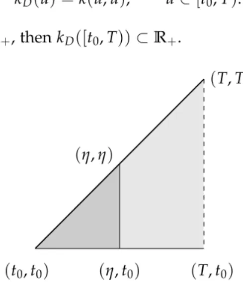
Let NandR+ denote, respectively, the sets of nonnegative integer and nonnegative real numbers. Lett0 ∈R andT ∈R∪ {∞}be such thatt0< T. Letc,r∈ R+,∆ := {(t,u)∈R2 : t0 ≤ u ≤ t < T}, D := {(t,u) ∈ ∆ : t = u} and∆η := {(t,u) ∈ ∆ : t ≤ η}, η ∈ [t0,T) (see Figure2.1). For a given functionk :∆→R, we define the functionkD :[t0,T)→Ras
kD(u) =k(u,u), u∈ [t0,T). It is obvious that if k(∆)⊂R+, thenkD([t0,T))⊂R+.
(η,t0) (η,η)
(t0,t0)
(T,T)
(T,t0)
Figure 2.1: The set∆. The subsetDis represented with a thick line. The subset
∆η, for someη∈[t0,T), is represented with darker colour.
Following the definitions in [5], measurability will refer to Lebesgue measurability, inte- grable will mean here Lebesgue integrable, thus we say that a function f :[t∗,T)→R, where t∗ ∈Ris such thatt∗ < T, is locally integrable if it is integrable over[t∗, ˆt], for every ˆt∈ [t∗,T).
Analogously, f is locally bounded if it is bounded on [t∗, ˆt], for every ˆt ∈ [t∗,T). We recall from [9] that the function ϕ : I → R, with I a real compact interval, is called absolutely continuous if, for everyε>0, there existsδ>0 such that
∑
n i=1|ϕ(βi)−ϕ(αi)|<ε
for anyn ∈Z, n≥1 and any disjoint set of intervals (α1,β1), . . . ,(αn,βn)⊂ I, whose lengths satisfy that
∑
n i=1(βi−αi)<δ.
Analogously, we will say that the function f :[t∗,T)→Ris locally absolutely continuous if it is absolutely continuous on each[t∗,t], for everyt ∈[t∗,T).
Finally, for each locally integrable mapping h : [t0−r,T) → R+, we define the function qh:[t0−r,T)→R+as
qh(t) =
Z t
t0
h(s)ds, t0−r≤ t< T.
In order to proof the results of the following section, we need some previous results. The first one is the Fundamental Theorem of Calculus for Lebesgue integration, which can be found in a large list of references such as [9].
Theorem 2.1. Let I be an interval of the real line and ϕ: I →Rbe an absolutely continuous function.
Then,ϕ0 exists almost everywhere (a.e.), it is integrable and ϕ(b) = ϕ(a) +
Z b
a ϕ0(s)ds, a,b∈ I.
In the following, the existence of derivatives of ϕin the whole interval will not be guar- anteed but, provided the hypotheses of the Fundamental Theorem of Calculus hold, we will refer to ϕ0 as some function defined in the same interval as ϕ, which can be extended to the remaining set of measure zero by defining it as needed.
Lemma 2.2. Letζ :∆→Rbe such thatζ(·,u): [u,T)→Ris locally absolutely continuous for each fixed u∈[t0,T). Moreover, suppose thatζD :[t0,T)→Ris locally integrable and that D1ζ :∆→R is integrable on each∆η, for allη∈[t0,T). Then, the following identity holds:
Z t
t0
ζ(t,u)du=
Z t
t0
ζ(u,u) +
Z u
t0
D1ζ(u,s)ds
du, t0 ≤t <T.
Proof. For eachu ∈ [t0,T), the function ζ(·,u)is locally absolutely continuous and, by Theo- rem2.1, D1ζ exists a.e. in∆. Hence, for a given(t,u)∈∆, we have
ζ(t,u) =ζ(u,u) +
Z t
u D1ζ(s,u)ds. (2.1)
Note that the integrability ofD1ζ on each∆η,η∈[t0,T), implies that y(u):=
Z t
u D1ζ(s,u)ds
is integrable inu. Then, if we integrate (2.1) betweent0andt, we reach to Z t
t0
ζ(t,u)du=
Z t
t0
ζ(u,u) +
Z t
u D1ζ(s,u)ds
du. (2.2)
Using the integrability ofD1ζ on each∆η, η∈[t0,T), we can change the order of variables of integration in (2.2) and obtain
Z t
t0
ζ(t,u)du=
Z t
t0
ζ(u,u)du+
Z t
t0
Z s
t0
D1ζ(s,u)duds. (2.3)
3 Volterra-type inequalities with delay dependence
In this section, we will present the principal results of this work. Theorems3.1and3.4provide the core of it, while Theorems3.6and3.8show that this type of results work in a more general framework.
Theorem 3.1. Let k : ∆ → R+ be such that k(·,u) : [u,T) → R is locally absolutely continuous for each fixed u ∈ [t0,T). Moreover, suppose that kD : [t0,T) → R+ is locally integrable and that D1k : ∆ → R+ is integrable on each ∆η, for all η ∈ [t0,T). Assume that τ : [t0,T) → R+ is a measurable function such that
t0−r ≤t−τ(t), t0 ≤t< T.
If x :[t0−r,T)→R+is Borel measurable and locally bounded such that x(t)≤c+
Z t
t0 k(t,u)x(u−τ(u))du, t0 ≤t< T, (3.1) then
x(t)≤Kexp Z t
t0
γ(s)ds
, t0≤t <T, (3.2)
where the functionγ:[t0−r,T)→R+is locally integrable and satisfies the characteristic inequality γ(t)≥k(t,t)exp
−
Z t
t−τ(t)γ(s)ds
+
Z t
t0
D1k(t,s)exp
−
Z t
s−τ(s)γ(w)dw
ds, (3.3) for t0≤ t<T a.e., and
K:=max (
cexp Z t
0
t0−rγ(s)ds
, sup
t0−r≤s≤t0
x(s) exp Z t
0
s γ(w)dw )
. Proof. First, we consider a continuousx in[t0,T).
Lety:[t0−r,T)→R+be defined as y(t) =x(t)exp
−
Z t
t0−rγ(s)ds
, t0−r ≤t< T.
Then, (3.1) implies that y(t)≤exp
−
Z t
t0−rγ(s)ds c+
Z t
t0
k(t,u)y(u−τ(u))exp
Z u−τ(u)
t0−r γ(s)ds
du
, for each t∈[t0,T). LetR:[t0,T)→R+ be defined as
R(t) =y(t−τ(t))exp
Z t−τ(t)
t0−r γ(s)ds
,
so we can write
y(t)≤exp
−
Z t
t0−r
γ(s)ds c+
Z t
t0
k(t,u)R(u)du
, t0≤ t<T.
Now we are going to apply Lemma2.2 to the functionζ(t,u) := k(t,u)R(u). First, ζ(·,u)is locally absolutely continuous due to the hypotheses ink. The function R is measurable and locally bounded and combined with the local integrability ofkD, we obtain thatζD is locally integrable. By a same reasoning, using the previous properties ofRand the hypotheses ink, one can conclude thatD1ζ is integrable in each∆η,η∈[t0,T). Then,
y(t)≤exp
−
Z t
t0−rγ(s)ds c+
Z t
t0
k(u,u)R(u) +
Z u
t0
D1k(u,s)R(s)ds
du
, for anyt∈ [t0,T). Taking
L:=max (
c, sup
u∈[t0−r,t0]
x(u)exp
−
Z u
t0−rγ(s)ds )
, we arrive, for anL1 > Larbitrarily chosen, to the following inequality:
y(t)≤ L< L1, t0−r≤ t≤t0.
Because of the continuity ofy, there exists an ε> 0 such thaty(t)< L1 fort ∈ [t0−r,t0+ε]. Suppose that there exists a t1 > t0+ε such that y(t1) = L1, which can be chosen as the first element satisfying this condition. Then,
L1 ≤cexp
−
Z t1
t0−rγ(s)ds
+L1exp
−
Z t1
t0
γ(s)ds
×
Z t1
t0
k(u,u)eqγ(u−τ(u))+
Z u
t0
D1k(u,s)eqγ(s−τ(s))ds
du. (3.4)
By using the characteristic inequality (3.3) in (3.4), we reach to L1 ≤cexp
−
Z t1
t0−rγ(s)ds
+L1exp
−
Z t1
t0
γ(s)ds Z t
1
t0
γ(u)eqγ(u)du.
By calculating the integral, we get L1 ≤cexp
−
Z t1
t0−rγ(s)ds
+L1
1−exp
−
Z t1
t0 γ(s)ds
. Then, rewriting terms, we obtain, by the choices ofLandL1, that
L1≤ L1+exp
−
Z t1
t0 γ(s)ds cexp
−
Z t0
t0−rγ(s)ds
−L1
< L1, which is a contradiction. We can assure thaty(t)≤ L, fort∈ [t0−r,T). Now,
x(t) =y(t)exp Z t
t0−rγ(s)ds
≤ Lexp Z t
t0−r
γ(s)ds
= Kexp Z t
t0
γ(s)ds
, t0≤ t< T.
To prove the result for the general case ofx, we proceed in the same way as in Theorem 2.2 [5].
Remark 3.2. The assumptions of Theorem1.3 (Theorem 2.2 [5]) are generalized by the ones in the previous theorem. If k(t,u) = f(u), for some locally integrable and nonnegative func- tion f, then this kernel satisfies all the hypotheses written in Theorem3.1. First, askdoes not depend on the first variable,k(·,u)is trivially locally absolutely continuous, for allu∈[t0,T), and D1k ≡ 0 in∆. Moreover,kD is locally integrable because kD(u) = k(u,u) = f(u), which is locally integrable by hypothesis. As a final comment, in Theorem3.1 inequality (3.3) is not imposed to be satisfied in every point of[t0,T).
As a consequence of Theorem 3.1, we derive the next result, which provides a simple estimate for the solutions of (3.1) through the use ofk.
Corollary 3.3. Let all the hypotheses of Theorem3.1hold. Then, x(t)≤Kexp
Z t
t0
k(t,s)ds
, t0≤t <T, where K is the same as in Theorem3.1.
Proof. By applying Lemma2.2to functionζ =k, we get Z t
t0
k(t,u)du=
Z t
t0
k(u,u) +
Z u
t0
D1k(u,s)ds
du, t0≤ t< T.
Now, one can conclude by choosing γ(t) =k(t,t) +
Z t
t0
D1k(t,s)ds, t0≤ t< T, and
γ(t) =0, t0−r≤t <t0. Indeed, it is obvious that γsatisfies (3.3).
The previous result provides an estimate for the solutions of the inequality (3.1) in terms of the function k(t,u), but it is not necessarily the best estimate. The next result states which is the sharpest one and how it is characterized.
Theorem 3.4. Let all the hypotheses of Theorem3.1hold. Then, the following assertions are valid.
1. There exists a unique locally integrable function γˆ : [t0−r,T) → R+ satisfying (3.3) with equality, for every t ∈[t0,T), and
ˆ
γ(t) =0, t∈[t0−r,t0). 2. Anyγ:[t0−r,T)→R+satisfying(3.3)also satisfies
ˆ
γ(t)≤γ(t), t0≤t <T.
3. The functionxˆ:[t0−r,T)→R+defined as ˆ
x(t) =cexp Z t
t0
ˆ γ(s)ds
, is the unique solution to the integral equation
x(t) =c+
Z t
t0
k(t,u)x(u−τ(u))du, t0≤t <T, with
x(t) =c, t0−r≤ t≤t0.
Proof. The proof is analogous to that of Theorem 2.7 [5]. We will only remark some points. To prove assertion1, we first extend the functionkto
D˜ :={(t,u)∈R2 :t0−r ≤u≤t <T} by defining
k(t,u) =0, (t,u)∈ D,˜ u∈ [t0−r,t0).
Then, we choose a sequence(γn)n∈Nof functions with domain[t0−r,T)defined as γ0(t) =k(t,t) +
Z t
t0 D1k(t,s)ds, t0−r≤ t<T, and then, by recurrence, forn∈N,
γn+1(t) =k(t,t)exp
−
Z t
t−τ(t)γn(s)ds
+
Z t
t0
D1k(t,u)exp
−
Z t
u−τ(u)γn(s)ds
du, for eacht0≤t <T and
γn+1(t) =0, t0−r≤t <t0.
Following the same reasoning of the proof of Theorem 2.7 in [5], one can assure that 0≤γ2k+1(t)≤γ2k+3(t)≤ · · · ≤γ2k+4(t)≤γ2k+2(t)≤γ0(t),
for anyk ∈Nandt ∈[t0−r,T). Then, by the Theorem of Dominated Convergence (see [9]), there exist
γup = lim
k→∞γ2k, and
γlow= lim
k→∞γ2k+1, and these limits satisfy
γup(t) =k(t,t)exp
−
Z t
t−τ(t)γlow(s)ds
+
Z t
t0
D1k(t,u)exp
−
Z t
u−τ(u)γlow(s)ds
du, (3.5) and
γlow(t) =k(t,t)exp
−
Z t
t−τ(t)γup(s)ds
+
Z t
t0 D1k(t,u)exp
−
Z t
u−τ(u)γup(s)ds
du.
fort0 ≤t< Tand
γup(t) =γlow(t) =0, t0−r ≤t<t0. By using that|e−x−e−y| ≤ |x−y|, forx,y≥0, we get to
0≤γup(t)−γlow(t)
=k(t,t)
Z t
t−τ(t)
[γup(s)−γlow(s)]ds+
Z t
t0
D1k(t,u)
Z t
u−τ(u)
[γup(s)−γlow(s)]dsdu, for anyt∈ [t0,T). By using the nonnegativity ofγup(t)−γlow(t), we can assure that
0≤γup(t)−γlow(t)≤
k(t,t) +
Z t
t0
D1k(t,u)du Z t
t0−r
[γup(s)−γlow(s)]ds.
By applying a simple Gronwall–Bellman inequality result (for example, see Theorem 1.3.2 [8]), we conclude that ˆγ := γup = γlowon [t0−r,T). It is clear that ˆγsatisfies (3.3) with equality because of the expresion (3.5). The uniqueness of ˆγ follows analogously to the procedure in [5], by using the same Gronwall–Bellman type result.
The second assertion can be proved in the same way as in [5].
It only remains to complete the proof of assertion3. Indeed, c+
Z t
t0 k(t,u)xˆ(u−τ(u))du= c+
Z t
t0 k(t,u)cexp
Z u−τ(u)
t0 γˆ(s)ds
du, (3.6)
and the last expression in (3.6) is equal to c+c
Z t
t0
k(u,u)eqγˆ(u−τ(u))+
Z u
t0 D1k(u,s)eqγˆ(s−τ(s))ds
du.
Using the characteristic inequality with equality in this case, the right-hand expression of (3.6) is also equal to
c
1+
Z t
t0
γ(u)eqγˆ(u)du
=ceqγˆ(t) =cexp Z t
t0
ˆ γ(s)ds
=xˆ(t).
In order to prove the uniqueness, one can reproduce similar arguments as those used in the proof of the first assertion, reaching an inequality of the type of (3.1), to which we can apply Theorem3.1.
In the following example we provide a family of functions k for which we can find the sharpest estimate.
Example 3.5. Let us consider
x(t)≤c+a(t)
Z
√t
1
√1
ux(u)du, t≥1. (3.7)
Then, after the substitutionu=√
zand renaming the variable, we obtain x(t)≤c+a(t)
Z t
1
1
2u34 x(u−(u−√
u))du, t ≥1.
In Example 3.5 (a) [5], the functionγ(t) = 2t1 provides the best estimate one could give for the solutions of (3.7) with a(t) =1. This remains true when
a(t) =1−Kexp
−
Z t
1
1 2(s−√
s)ds
,
for anyK∈ [0, 1]. This can be proved by checking that (3.3) holds with equality a.e. on[1,∞) and, then, Theorem3.4can be applied.
Now, we show some generalizations of Theorem3.1. The first one is related to the solutions to another inequality of the type of (3.1), which has another integral term (without “delay”) on the right-hand side.
Theorem 3.6. Let k,g : ∆ → R+ be such that k(·,u),g(·,u) : [u,T) → R are locally absolutely continuous for each fixed u ∈ [t0,T). Moreover, let kD,gD : [t0,T) → R+ be locally integrable and such that D1k,D1g : ∆ → R+ are integrable on each ∆η, for all η ∈ [t0,T). Assume that τ:[t0,T)→R+is a measurable function such that
t0−r ≤t−τ(t), t0≤t <T.
If x:[t0−r,T)→R+is Borel measurable and locally bounded such that x(t)≤c+
Z t
t0
g(t,u)x(u)du+
Z t
t0
k(t,u)x(u−τ(u))du, t0≤ t<T, (3.8) then
x(t)≤Kexp Z t
t0
γ(s)ds
, t0≤ t<T, (3.9)
where the functionγ:[t0−r,T)→R+is locally integrable and satisfies the characteristic inequality γ(t)≥k(t,t)exp
−
Z t
t−τ(t)
[γ(w) +g(t,w)]dw
+
Z t
t0
D1k(t,s)exp
−
Z t
s−τ(s)
[γ(w) +g(s,w)]dw
ds, (3.10)
for t0 ≤t< T a.e., and K is equal to max
( cexp
Z t
0
t0−rγ(s)ds
, sup
t0−r≤s≤t0
x(s)exp Z t
0
s γ(w)dw )
. (3.11)
Proof. The key point of the proof will be to manipulate the inequality (3.8) in order to reach an expression which satisfies Theorem3.1.
In the appendix (Lemma6.1) we prove that x(t)≤cexp
Z t
t0 g(t,u)du
+exp Z t
t0
g(t,u)du Z t
t0
k(t,u)x(u−τ(u))exp
−
Z u
t0
g(u,s)ds
du, (3.12) for eacht∈ [t0,T). Then, by defining
G(t):= g(t,t) +
Z t
t0
D1g(t,s)ds, (3.13)
and
y(t):= x(t)exp
−
Z t
t0 G(s)ds
, it is possible to rewrite (3.12) as
y(t)≤c+exp
−
Z t
t0 G(s)ds Z t
t0 k(t,u)y(u−τ(u))exp
Z u−τ(u)
t0 G(s)ds+
Z t
u G(s)ds
du, or equivalently,
y(t)≤c+
Z t
t0
k(t,u)y(u−τ(u))exp
−
Z u
u−τ(u)G(s)ds
du.
Now, by using analogous arguments as in the beginning of the proof for Theorem 3.1, the function
ψ(t,u):=k(t,u)exp
−
Z u
u−τ(u)G(s)ds
=k(t,u)exp
−
Z u
u−τ(u)g(t,s)ds
can play the role ofk in Theorem3.1and y(t)≤Kexp
Z t
t0
γ(s)ds
, t0 ≤t< T, whereγ:[t0−r,T)→R+satisfies
γ(t)≥ψ(t,t)exp
−
Z t
t−τ(t)γ(w)dw
+
Z t
t0
D1ψ(t,s)exp
−
Z t
s−τ(s)γ(w)dw
ds andKis as (3.11).
Remark 3.7. In the proof of the previous theorem, by some calculations, we have used the thesis of Theorem 3.1. Therefore, by a parallel way, the assertions of Theorem 3.4 can be adapted to this case, and one can see the optimality properties of the unique function ˆγthat satisfies (3.10) with equality.
Finally, as done in [5], it is possible to substitute c by a positive, measurable and nonde- creasing function with the goal of obtaining an analogous result to the previous ones.
Theorem 3.8. Let p:[t0,T)→R+be a measurable, positive and (monotone) nondecreasing function.
Let k,g : ∆ → R+ be such that k(·,u),g(·,u) : [u,T) → R are locally absolutely continuous for each fixed u ∈ [t0,T). Moreover, suppose that kD,gD : [t0,T) → R+ are locally integrable and D1k,D1g :∆→R+ are integrable on each∆η, for allη∈ [t0,T). Assume thatτ:[t0,T)→R+is a measurable function such that
t0−r ≤t−τ(t), t0 ≤t< T.
If x :[t0−r,T)→R+is Borel measurable and locally bounded such that x(t)≤ p(t) +
Z t
t0
g(t,u)x(u)du+
Z t
t0
k(t,u)x(u−τ(u))du, t0≤ t<T, (3.14) then
x(t)≤Kp(t)exp Z t
t0
γ(s)ds
, t0 ≤t< T, (3.15)
where the functionγ:[t0−r,T)→R+is locally integrable and satisfies the characteristic inequality γ(t)≥k(t,t)exp
−
Z t
t−τ(t)
[γ(w) +g(t,w)dw]
+
Z t
t0
D1k(t,s)exp
−
Z t
s−τ(s)
[γ(w)dw+g(s,w)]dw
ds, (3.16)
for t0≤ t<T a.e., and K :=max
( exp
Z t
0
t0−rγ(s)ds
, sup
t0−r≤s≤t0
x(s) p(s) exp
Z t
0
s γ(w)dw )
.
Proof. The proof follows by dividing by p(t)in (3.14) and applying Theorem 3.6 with c = 1 and the function
z(t):= x(t) p(t) playing the role ofx in that result.
4 An application to functional differential equations
The results of the previous sections can be employed to study some types of functional differ- ential equations. In particular, some equations with an integral term can be included in our framework. For example, consider the functional differential equation
x0(t) =−2
tx(t)− 1 4t2x
1 2
√ t
+
Z t
1
1 4t2sx
1 2
√s
ds, t ≥1. (4.1)
We will see that all solutions to (4.1) tend to 0 as t → ∞. By integrating and applying analogous arguments to those of the Appendix, we get
x(t) =x(1)exp
−
Z t
1
2 sds
+exp
−
Z t
1
2 sds
Z t
1
− 1 4s2x
1 2
√s
+ 1
4s2u Z s
1 x 1
2
√u
du
exp Z s
1
2 wdw
ds.
This leads to
x(t) = x(1) t2 + 1
t2 Z t
1
−1 4x
1 2
√s
+
Z s
1
1 4ux
1 2
√u
du
ds. (4.2)
If we define
y(t):=t2x(t), we can substitute in (4.2) and obtain
y(t) =y(1) +
Z t
1
−1 sy
1 2
√s
+
Z s
1
1 u2y
1 2
√u
du
ds.
Then,
|y(t)| ≤ |y(1)|+
Z t
1
1 s y
1 2
√s
+
Z s
1
1 u2
y
1 2
√u
du
ds. (4.3)
By applying Lemma2.2, we can write (4.3) as
|y(t)| ≤ |y(1)|+
Z t
1
t s2
y
1 2
√s
ds, whereζ =k(t,s)|y(12√
s)|, for
k(t,s) = t s2,
which is included in the framework of Theorem3.1. Now, we can choose any locally integrable functionγ:[12,∞)→R+such that
γ(t):= 1
t, t≥1.
It can be checked by some calculations that the generalized characteristic inequality (3.3) holds for this case, i.e.,
1 t ≥ 1
t exp
−
Z t
1 2
√t
1 sds
+
Z t
1
1 u2exp
−
Z t
1 2
√u
1 sds
du.
Then, we can assure that there exists someK∈R+such that
|y(t)| ≤Kexp Z t
1 γ(s)ds
=Kexp Z t
1
1 sds
=Kt, t≥1.
Then,
|x(t)| ≤ K
t , t≥1, which obviously leads to
tlim→∞x(t) =0.
The classical estimate that Corollary3.3provides is
|y(t)| ≤K0exp Z t
1 k(t,s)ds
=K0exp Z t
1
t s2ds
=K0et−1, t ≥1,
for some K0 ∈ R+. The previous estimate is not good enough to assure global attractiv- ity of 0, so this example shows the importance of results like Theorem 2.2 [5] or Theorem 3.1. The reason is they provide more functions (than the classical estimates with f(u) and k(t,u), respectively) from which we can “build” estimates for the solutions to certain integral inequalities.
5 Conclusion
In this work, we have presented some generalizations of the results of [5] and some classical results as Theorems 1.1 and 1.2. Theorems 3.1 and 3.4 represent the central part of the ex- posed contents and provide, respectively, estimates for the solutions to the integral inequality (3.1) and their sharpness properties. Finally, we have proposed an example of a functional differential equation (with an integral term) whose stability properties are derived from the aforementioned results.
6 Appendix
In this appendix, we give the proof of a certain step (related to auxiliar estimates) in the proof of Theorem3.6.
Lemma 6.1. Let the hypotheses of Theorem3.6hold. Then, x(t)≤cexp
Z t
t0 g(t,u)du
+exp Z t
t0
g(t,u)du Z t
t0
k(t,u)x(u−τ(u))exp
−
Z u
t0
g(u,w)dw
du, (6.1) for each t0≤ t<T.
Proof. Definezas the right-hand side of (3.8). This function is absolutely continuous on each [t0,t∗]. Then, z is differentiable almost everywhere, i.e., on some set Ωt∗, with [t0,t∗]\Ωt∗ having zero measure. Besides,
z0(t) =g(t,t)x(t) +
Z t
t0
D1g(t,u)x(u)du +k(t,t)x(t−τ(t)) +
Z t
t0 D1k(t,u)x(u−τ(u))du, t∈Ωt∗,
and usingx(t)≤z(t)fort∈ [t0,t∗], then z0(t)≤ g(t,t)z(t) +
Z t
t0 D1g(t,u)z(u)du +k(t,t)x(t−τ(t)) +
Z t
t0
D1k(t,u)x(u−τ(u))du, t∈ Ωt∗. (6.2) Asz(u)≤z(t), foru∈ [t0,t]a.e., we can assure that
z(t)exp
−
Z t
t0
g(t,u)du 0
≤
z0(t)−g(t,t)z(t)−
Z t
t0
D1g(t,u)z(u)du
×exp
−
Z t
t0
g(t,u)du
, t∈ Ωt∗. (6.3) Then, by using (6.2) and (6.3), we get
z(t)exp
−
Z t
t0
g(t,u)du 0
≤
k(t,t)x(t−τ(t)) +
Z t
t0
D1k(t,u)x(u−τ(u))du
(6.4)
×exp
−
Z t
t0
g(t,u)du
, t ∈Ωt∗. By integrating (6.4) betweent0 andt∗, we reach to
z(t)exp
−
Z t
t0
g(t,u)du
−z(t0)
≤
Z t
t0
k(s,s)x(s−τ(s)) +
Z s
t0
D1k(s,u)x(u−τ(u))du
(6.5)
×exp
−
Z s
t0
g(s,w)dw
ds, t∈[t0,t∗].
Now, if we use the nonnegativity ofgandD1g, then the right-hand side of (6.5) is less than or equal to
Z t
t0
k(s,s)x(s−τ(s))exp
−
Z s
t0
g(s,w)dw
ds +
Z t
t0
Z s
t0
D1k(s,u)x(u−τ(u))exp
−
Z u
t0
g(u,w)dw
duds. (6.6)
Then, by using Lemma2.2 withζ being defined as ζ(t,u) =k(t,u)x(u−τ(u))exp
−
Z u
t0
g(u,w)dw
, (6.6) is equivalent to
Z t
t0
k(t,u)x(u−τ(u))exp
−
Z u
t0
g(u,w)dw
du.
Following this previous reasoning, (6.5) leads to z(t)≤cexp
Z t
t0
g(t,u)du
+exp Z t
t0
g(t,u)du Z t
t0
k(t,u)x(u−τ(u))exp
−
Z u
t0
g(u,w)dw
du,
where we have used z(t0) = c. Now the result follows from the definition ofz (x(t) ≤ z(t), for any t∈[t0,T)) and from the fact thatt∗ was arbitrarily chosen in[t0,T).
Acknowledgements
The authors thank Prof. Eduardo Liz for all his kind suggestions for the improvement of the manuscript. They also acknowledge all the valuable comments coming from the reviewing process.
This research was partially supported by Agencia Estatal de Investigación of Spain (un- der grant MTM2016-75140-P, cofunded by European Community fund FEDER) and Con- sellería de Cultura, Educación e Ordenación Universitaria da Xunta de Galicia (under grants GRC2015/004 and R2016-022).
Ministerio de Educación, Cultura y Deporte of Spain (grant FPU16/04416) and Con- sellería de Cultura, Educación e Ordenación Universitaria da Xunta de Galicia (grant ED481A- 2017/030) also partially supported the research of Sebastián Buedo-Fernández.
References
[1] K. Ahmedov, M. Jakubov, I. Veisov, Some integral inequalities, Izv. Akad. Nauk. UZSSR 1(1972), 18–24.
[2] R. Bellman, The stability solutions of linear differential equations, Duke Math. J.
10(1943), 643–647. https://doi.org/10.1215/S0012-7094-43-01059-2; MR0009408;
Zbl 0061.18502
[3] S. S. Dragomir,Some Gronwall type inequalities and applications, Nova Science Publishers, New York, 2003.MR2016992;Zbl 1094.34001
[4] T. H. Gronwall, Note on the derivatives with respect to a parameter of the solutions of a system of differential equations,Ann. of Math.20(1919), 292–296.https://doi.org/10.
2307/1967124;MR1502565;Zbl 47.0399.02
[5] I. Gy ˝ori, L. Horváth, Sharp Gronwall–Bellman type integral inequalities with delay,Elec- tron. J. Qual. Theory Differ. Equ.2016, No. 111, 1–25.https://doi.org/10.14232/ejqtde.
2016.1.111;MR3582904;Zbl 06837987
[6] I. Gy ˝ori, L. Horváth, Sharp estimation for the solutions of delay differential and Halanay type inequalities. Discrete Contin. Dyn. Syst. 37(2017), 3211–3242. https://doi.org/10.
3934/dcds.2017137;MR3622080;Zbl 06694020
[7] J. Norbury, A. M. Stuart, Volterra integral equations and a new Gronwall inequality.
Part I: the linear case,Proc. Roy. Soc. Edinburgh Sect. A106(1987), 361–373.https://doi.
org/10.1017/S0308210500018473;MR0906218;Zbl 0639.65075
[8] B. G. Pachpatte, Inequalities for differential and integral equations, Mathematics in Science and Engineering, Vol. 197, Academic Press, San Diego, 1998.MR1487077;Zbl 1032.26008 [9] W. Rudin,Real and complex analysis, 3rd ed., McGraw-Hill International Editions, Singa-
pore, 1987.MR924157