On the global attractor of delay differential equations with unimodal feedback not satisfying the negative
Schwarzian derivative condition
Dedicated to Professor Jeffrey R. L. Webb on the occasion of his 75th birthday
Daniel Franco
B1, Chris Guiver
2, Hartmut Logemann
3and Juan Perán
11Departamento de Matemática Aplicada, E.T.S.I. Industriales, Universidad Nacional de Educación a Distancia (UNED), c/ Juan del Rosal 12, Madrid, 28040, Spain
2School of Engineering & the Built Environment, Edinburgh Napier University, Merchiston Campus, Edinburgh, EH10 5DT, UK
3Department of Mathematical Sciences, University of Bath, Claverton Down, Bath, BA2 7AY, UK
Received 24 June 2020, appeared 21 December 2020 Communicated by Tibor Krisztin
Abstract. We study the size of the global attractor for a delay differential equation with unimodal feedback. We are interested in extending and complementing a dichotomy result by Liz and Röst, which assumed that the Schwarzian derivative of the nonlinear feedback is negative in a certain interval. Using recent stability results for difference equations, we obtain a stability dichotomy for the original delay differential equation in the situation wherein the Schwarzian derivative of the nonlinear term may change sign. We illustrate the applicability of our results with several examples.
Keywords: delay differential equations, difference equations, global attractor.
2020 Mathematics Subject Classification: 39B82, 39A30.
1 Introduction
The nonlinear delay differential equation x′(t) =−µ(
x(t)− f(x(t−τ))), t>0, (1.1) with µ,τ > 0 and f: I ⊂ R → I, has been widely studied in the literature because of its multiple applications in, for example, biology, physics or economics [1,2,14,17]. In the case of f being monotone, the dynamics are well understood, see [8,9,18] and references therein. In particular, it is known that chaotic dynamics cannot occur [15]. The natural generalization of
BCorresponding author. Email: dfranco@ind.uned.es
the previous case, in which f changes monotonicity once, is more complicated and may lead to chaotic behaviour [10].
In this paper, f is assumed to be unimodal. More specifically, we impose that the following condition holds for f.
(U) f: (a,b)⊂R →(a,b)is differentiable, with−∞≤ a< b≤ +∞; satisfies that there is a uniquex∗ such that f′(x)>0 ifa≤ x< x∗, f′(x∗) =0, and f′(x)<0 ifx∗ <x <b; and that there existsK ∈ (x∗,b)such that f(K) = K, f(x) > x for x ∈ (a,K), and f(x) < x forx∈(K,b).
Notice that if condition(U)holds, thenKis the uniquefixed pointfor the map f, i.e. f(K) =K, and therefore the constant function x(t) = K is a positive equilibrium of the delay equa- tion (1.1). Moreover, we empshasise that assuming that the fixed pointK belongs to(x∗,b)is not restrictive for our purpose of studying the asymptotic behaviour of equation (1.1), since if K belongs to the interval(a,x∗), then all the solutions of the delay equation are known to converge toK; see, for example [16].
Whenever condition(U)holds, we denote the image by f of the point where the maximum of f is attained and the image by f of this maximum by βandα, respectively, that is,
β:= f(x∗) and α:= f(β). (1.2) With the notation in (1.2), we introduce an additional assumption on f.
(L) Condition(U)holds and f(f(x∗))>x∗.
A well-known approach for investigating equation (1.1) comprises studying the behaviour of the related difference equation
xn+1= f(xn), x0 ∈(a,b), (1.3) see, for example, [7,13]. Using that approach and taking advantage of the properties of unimodal maps it is possible to show that if(L)holds, then for any solutionx(t)of (1.1) with initial condition inC([−τ, 0],(a,b))there existst0>0 such thatx(t)∈[α,β]fort≥t0; and we informally say that the interval[α,β]contains the global attractor of the equation (1.1). Thus, if(L)holds, then the interval [α,β]contains the global attractor of (1.1) independently of the delayτ. Moreover, complicated dynamics cannot occur for equation (1.1) since theω-limit set of any solution is the positive equilibrium{K}or a periodic orbit. We refer the reader to [16]
for a proof of these results in the particular case of(a,b) = (0,+∞).
The interval [α,β] might not be the sharpest, that is, it might have a proper subinterval which contains the global attractor of (1.1). Therefore, an interesting problem stated in [16]
is to try to estimate this sharpest attracting interval—or even better to calculate it—when condition(L)holds. Here, we deal with such a problem.
In [11], Liz and Röst consider the same problem and showed that when f satisfies (L) and has negative Schwarzian derivative, then the sharpest interval containing the attractor of equation (1.1) can be determined and the following dichotomy result holds.
Theorem 1.1(Theorem 6 in [11]). Assume that condition(L)holds and, further, that f satisfies the following condition.
(S) f is three times differentiable and (S f)(x) < 0 on the interval [α,β], where S f denotes the Schwarzian derivative of f , defined by
(S f)(x) = f
′′′(x) f′(x) −3
2
(f′′(x) f′(x)
)2 . Then exactly one of the following holds:
1. f′(K)≥ −1and the global attractor of (1.1)for all values of the delayτis{K}.
2. f′(K) < −1 and the sharpest invariant and attracting interval containing the global attractor of (1.1) for all values of the delayτis[α, ¯¯ β], where{α, ¯¯ β}is the unique nontrivial 2-cycle (i.e., α¯ = f(β¯)andβ¯ = f(α¯)) of the map f in[α,β].
Remark 1.2. We note that Theorem1.1as stated above is, in fact, a slightly generalized version of Theorem 6 in [11], which follows from the ideas in [11]. Specifically, the result by Liz and Röst is stated for the particular case in whicha=0 andb= +∞. Moreover, their condition (U) imposes f′′(x) > 0 on (0,x∗), but this is just to guarantee that f has a unique positive fixed point. We note that under the conditions in [11], f: [0,+∞) → [0,+∞) is continuous and satisfies f(0) = 0 and f(x) > 0 for x > 0, hence, the restriction to the open interval (0,+∞) that we consider in Theorem1.1 is well defined. Finally, note that the initial condition in [11]
is a nonzero and nonnegative real function on [−τ, 0]and consequently all the solutions are strictly positive fort>0, as remarked there. Hence, there is no loss of generality in assuming the initial condition to be strictly positive as we do here.
As the authors of [11] highlighted, the function f appearing in important examples of equation (1.1), including the Mackey–Glass and Nicholson’s blowflies models [6,12], does have negative Schwarzian derivative. Nevertheless, it is not hard to find situations where (S) does not hold and, therefore, Theorem1.1is not applicable. Hence, it is interesting to look for results extending and complementing Theorem1.1.
In order to obtain such results, without the assumption that f has negative Schwarzian derivative, we instead take advantage of a consequence of (L), namely, that f|(α,β) is strictly decreasing. In this case, the recent method presented in [4,5] for studying the dynamics of difference equations is applicable, and we employ it to establish a dichotomy result for (1.1) by studying (1.3). Proposition 2.6 is the key technical ingredient for the difference equations we consider, and our main result is Theorem3.2. The latter result has the same conclusions of Theorem1.1, but different hypotheses.
Interestingly, the proof of Proposition 2.6 uses the second inequality in the Hermite–
Hadamard inequality for a strictly convex functionh: [a,b]→R, h
(a+b 2
)
< 1
b−a
∫ b
a h(x)dx< h(a) +h(b)
2 , (1.4)
to show that certain function, intimately linked to the dynamics of the difference equation, is strictly increasing. Whereas, for guaranteeing that such a function has a strict global minimum—enough for obtaining the first conclusion in Theorem 1.1—one needs to invoke the first inequality in (1.4).
In recognition of the current special volume, Professor Webb is a world-expert on the use of topological tools in the study of nonlinear problems. Indirectly, fixed point index theory applied to the study of differential equations plays a role in this paper. Indeed, this is one
of the tools used by Mallet-Paret and Nussbaum in [13] to prove the existence of slowly oscillating periodic solutions. The properties of those slowly oscillating periodic solutions underpin [11, Proposition 5], which we invoke in the proof of our main result.
The rest of the paper is organized as follows. The next section contains the preliminaries:
notation and some stability results for difference equations. Section 3 contains our main results. Finally, last section of the paper includes some examples to illustrate these main results and compare them with Theorem1.1.
2 Preliminaries
2.1 Notation
As usualNandR denote the positive integers (natural numbers) and real numbers, respec- tively. Furthermore,R+:={r∈R : r≥0}.
LetI ⊂Rbe an interval (bounded or unbounded) and f a continuous map from Ito itself.
We denote
f(0):=id, f(n+1)= f◦f(n), n≥1, n∈N, with id denoting the identity map; i.e., id(x) =xfor all x∈ I.
We letCn(J,I)denote the space of functionsξ: J →I withncontinuous derivatives and, to simplify the notation,Cn((a,b),R)is denoted by Cn(a,b):= Cn((a,b),R)when no confusion is possible. We do not explicitly indicate the domains of the identity and constant functions.
They are assumed to be the largest sets for which the corresponding expressions make sense.
We say that x(t;ξ)is a solution of the differential equation (1.1) with f ∈ C(R)and initial conditionξ ∈ C([−τ, 0],R)if x(·;ξ) ∈ C([−τ,+∞),R), x(·;ξ)|(0,+∞) ∈ C1(0,+∞), it satisfies the differential equation (1.1) fort>0 and x(s;ξ) =ξ(s)fors∈[−τ, 0]. The method of steps, e.g., see [17], shows that there exists a unique solution of the differential equation (1.1) for any f ∈ C(R)and initial conditionξ ∈ C([−τ, 0],R). Moreover, if f ∈ C(I,I)andξ ∈ C([−τ, 0],I), then the invariance principle (see [7, Theorem 2.1]) guarantees that the unique solution of (1.1) satisfiesx(t;ξ)∈ I for all t∈[−τ,+∞).
2.2 Stability of difference equations
In this section, we study stability properties of the difference equation
yn+1= yn+g(yn), y0∈dom g, (2.1) withg∈G, where
G:= ∪
−∞≤a<b≤∞
G(a,b), and
G(a,b):= {g∈ C1(a,b) : a <id+g <b, g′ <0, 0∈g(
(a,b))}. Hereg(
(a,b))denotes the image of(a,b)underg. It is clear that for eachg∈G∗the difference equation (2.1) is well defined and there exists a unique yg ∈ (a,b) such that g(yg) = 0. In particular, yg is a unique equilbrium of (2.1). We use the usual definitions of stability, local asymptotic stability and global asymptotic stability for the equilibrium yg of the difference equation (2.1). From now on, G.A.S. stands for globally asymptotically stable and L.A.S. for locally asymptotically stable. We state what we understand by a global repeller.
Definition 2.1. We say that yg is a a global repeller for the difference equation (2.1) if the sequence ((id+g)(n)(y))n has no accumulation points in(a,b)for anyy ∈(a,b)\yg.
Next, we define a function to study the stability properties of the equilibrium of (2.1), which was introduced in [5].
Definition 2.2. For each g ∈ G, set bg := min{−infg, supg}. The function σg: (−bg,bg) → (0,+∞)is defined by
σg(u) =
g−1(−u)−g−1(u)
u ifu̸=0 ,
−2
g′(yg) ifu=0 . The following remark will be very useful in this section.
Remark 2.3. Since(g−1)′ is continuous,σg satisfies σg(u) = 1
u
∫ u
−u−(g−1)′
(s)ds ∀u∈ (0,bg).
The function σg is continuous, even and positive. Moreover, y ∈ domg\yg satisfies (id+g)(2)(y) = yif, and only if, u= g−1(y)∈ domσg satisfiesσ(u) = σ(−u) =1, see [5]. In other words, the nontrivial period-2 solutions of (2.1) correspond to the symmetric intersec- tions of the graph ofσg with the the graph of the constant function with value 1.
Our next result shows that the stability properties ofygare intimately linked to the relative position of the functionσg with respect to the constant function with value 1.
Theorem 2.4. Let g ∈G. The following statements hold for the unique equilibrium ygof (2.1):
a) yg is L.A.S. ifσg(0)>1, and it is unstable ifσg(0)<1.
b) yg is G.A.S. if, and only if,σg(u)>1for all u∈ (−bg,bg)\ {0}. c) Ifσg(u)≥1for all u in a neighbourhood of u =0, then yg is stable.
d) Ifσg(u)<1for all u in a punctured neighbourhood of u=0, then ygis unstable.
e) yg is a global repeller if, and only if,σg(u)<1for all u∈(−bg,bg)\ {0}. f) Ifσg(u)>1for all u in a punctured neighbourhood of u=0, then ygis L.A.S.
Proof. The proof of statementsa)–d) can be found in [5]. Similar ideas can be used to prove statementse)andf). Indeed, the reader just needs to reverse the inequalities in the proof ofb) and to invoke [5, Proposition 4.d] to obtain the proof ofe); whereas reversing the inequalities ind) and invoking [5, Proposition 3.a] gives the proof off).
Our next result illustrates how Theorem2.4can be used to obtain sufficient conditions for the (in)stability of the equilibriumyg of the difference equation (2.1).
Proposition 2.5. Let g ∈G. The following statements hold.
a) If g′(y)<−2for all y∈(a,b)\{yg}, then ygis a global repeller for(2.1).
b) If g′(y)>−2for all y∈(a,b)\{yg}, then ygis G.A.S. for(2.1).
Proof. To prove statementa), we argue that
σg(u)<1 ∀u∈(0,bg), (2.2) and invoke statemente)of Theorem2.4, combined with the property thatσgis an even func- tion.
For which purpose, recalling that (g−1)′
(u) = 1
g′(g−1(u)) ∀u∈(−bg,bg), our hypothesis ongin statementa)implies that
−(g−1)′
(u)< 1
2 ∀u∈ (−bg,bg)\{0}. Therefore, recalling Remark2.3,
σg(u) = 1 u
∫ u
−u−(g−1)′
(s)ds<1 ∀u∈(0,bg), and so (2.2) holds.
The proof of statementb)is similar, and argue that σg(u)>1 ∀u∈(0,bg),
which, when combined with statementb)of Theorem2.4, proves the claim.
Proposition 2.6. Let g∈G. The following statements hold.
a) If( g−1)′
is strictly convex or strictly concave, then the difference equation(2.1)has at most one nontrivial period-2 solution.
b) If( g−1)′
is strictly convex and g′(yg)≤ −2, then ygis a global repeller for(2.1).
c) If( g−1)′
is strictly concave and g′(yg)≥ −2, then ygis G.A.S. for(2.1).
Noting that
(g−1)′′′(u) = 3(g′′(y))2−g′(y)g′′′(y)
(g′(y))5 ∀u =g(y), y∈(a,b), a sufficient condition for strict convexity (concavity) of(
g−1)′
in the case that g ∈ C3(dom g) is that
3(g′′)2−g′g′′′ (2.3)
is negative (positive).
Proof of Proposition2.6. We claim that if g−1 is strictly convex (concave), then the function σg
is strictly decreasing (increasing) on the interval (0,bg). Assuming this, strict monotonicity of σg implies that there is at most one solution of 1 = σg(u) in (0,bg), and so invoking the properties ofσg recalled after Definition2.2, we conclude that (2.1) has at most one nontrivial period-2 solution, proving statementa).
Thus, if ( g−1)′
is strictly convex, then Remark 2.3 and an application of the second Hermite–Hadamard inequality in (1.4) yields
u d
duσg(u) =u d du
(−1 u
∫ u
−u
(g−1)′(s)ds )
= 1 u
∫ u
−u
(g−1)′(s)ds−((g−1)′(−u) + (g−1)′(u)) <0 ∀u∈(0,bg), that is,σg′ <0 and so σg is strictly decreasing on(0,bg).
Analogously, if(g−1)′ is strictly concave, then −(g−1)′ is strictly convex and so
−u d
duσg(u) =u d du
(−1 u
∫ u
−u−(g−1)′(s)ds )
= 1 u
∫ u
−u−(g−1)′(s)ds−(−(g−1)′(−u) +−(g−1)′(u)) <0 ∀u∈ (0,bg). that is, σg′ > 0. We conclude thatσg is strictly increasing on(0,bg). The proof of statementa) is complete.
Under the hypotheses in statementb), that (2.2) holds is clear upon noting that σg(0) =
−2/g′(yg) ≤ 1 and that we have just shown in proof of statement a) that σg is strictly in- creasing on the interval (0,bg). Invoking statemente)of Theorem2.4 completes the proof of statementb).
Reasoning analogous to that used in the proof of statementb)proves statementc), and so we omit the details.
Remark 2.7.
(i) If ( g−1)′
is strictly convex, then using the first Hermite–Hadamard inequality in (1.4) gives
σg(u) = −1 u
∫ u
−u
(g−1)′(s)ds<−2(g−1)′(0) = −2
g′(yg) =σg(0) ∀u∈ (0,bg), and, consequently, σg attains a global maximum at 0. Hence, statement b) in Proposi- tion 2.6 may be proven by statement e) of Theorem 2.4 directly together with the first inequality in the Hermite–Hadamard inequality, instead of the second inequality as was done above. A similar comment is valid for statementc)of Proposition2.6.
(ii) Assume thatbg = +∞. Since (g−1)′
(u) = 1
g′(g−1(u)) <0 ∀u ∈(−∞,+∞), as g is strictly decreasing, it follows that −(g−1)′
(u) > 0. In particular, if ( g−1)′
is convex in R, then −(g−1)′
is concave and positive in R, and hence must be constant.
Therefore,( g−1)′
cannot be strictly convex. This implies that (2.3) cannot be negative.
In light of the above, whenbg = +∞, statementb) of Proposition2.6cannot be applied.
We finish the section by showing how Theorem 2.4 and Proposition 2.6 can be used to study a particular type of positive difference equation via topological conjugacy. We define
C:= ∪
−∞≤a<b≤∞
C(a,b) and C+ := ∪
0≤a<b≤∞
C+(a,b),
withC+(J) ={d ∈ C(J): d > 0}, and define T:C+ →C byT(d) =ln◦d◦exp. Clearly,Tis bijective, with inverseT−1: C→C+given byT−1(g) =exp◦g◦ln. Define
D:=T−1(G) = ∪
0≤a<b≤∞
D(a,b), with
D(a,b):={d∈ C1(a,b):a<id·d<b, d′ <0, 1∈ d(
(a,b))}, and consider the difference equation
xn+1 =xnd(xn), x0∈domd, (2.4) whered∈ D. Note that for eachd∈ Dthere exists a unique xd ∈domd such thatd(xd) = 1, and consequentlyxd is an equilibrium of (2.4).
A routine calculation shows that x = (xn) is a solution of (2.1) if, and only if, z = ex is a solution of (2.4), where g and d are related by d = T−1(g). Therefore, stability properties of (2.4) may be studied by applying Theorem 2.4 and Proposition 2.6 to the transformed version (2.4).
3 Sharpest interval containing the attractor
We will make use of the following result (see [7, Theorems 2.2 and 2.3]).
Lemma 3.1. If there exists an interval I0⊂ I such that infI0≤lim inf
n→+∞ f(n)(x)≤lim sup
n→+∞
f(n)(x)≤supI0 ∀x∈ I, then the solutions of (1.1)satisfy
infI0≤lim inf
t→+∞ x(t,ξ)≤lim sup
t→+∞
x(t,ξ)≤supI0 ∀τ>0, ∀ξ ∈ C([−τ, 0],I). In particular, if K is G.A.S. for the difference equation(1.3), then
t→lim+∞x(t;ξ) =K ∀τ>0, ∀ξ ∈ C([−τ, 0],I).
The following theorem is the main result of this paper. It provides a partial answer to the problem of finding the sharpest attracting interval for the delay-differential equation (1.1) under condition(L)by establishing a dichotomy, in the flavour of that of Theorem1.1.
Theorem 3.2. Assume that(L)holds, that f is three times differentiable and satisfies
3(f′′)2−(f′−1)f′′′ >0 , (3.1) on the interval(α,β). Then exactly one of the following holds:
1. f′(K)≥ −1and the global attractor of (1.1)for all values of the delayτis{K}.
2. f′(K) < −1and the sharpest invariant and attracting interval containing the global attractor of (1.1)for all values of the delayτis[α, ¯¯ β], where{α, ¯¯ β}is the unique nontrivial 2-cycle of the map f in[α,β].
Proof. Using condition(L), it is not hard, but tedious since several cases need to be considered, to see that for anyx0∈ I there existsn ∈Nsuch that f(n)(x0)∈(α,β), and f([α,β])⊂ [α,β).
Defineg := f−id. We claim that g belongs toG(α,β). To see this, note that g is strictly decreasing in[α,β]since f is. Also, note that
g(x) +x = f(x)∈(α,β) ∀x ∈(α,β) and, since f([α,β])⊂[α,β),
f(β)−β<0< f(α)−α, so 0∈ g(
(α,β)), and we have thatg∈G(α,β).
Assume first that f′(K) ≥ −1. Using that for any x0 ∈ I there exists n ∈ N such that f(n)(x0) ∈ (α,β)and invoking the second part of Lemma 3.1, it is enough to show that K is G.A.S. for the difference equation (2.1). And this follows from the second part of Proposi- tion 2.6 after noting that g′(K) ≥ −2, because f′(K) ≥ −1, and that the function in (2.3) is positive, because (3.1) holds.
Assume now that f′(K)<−1. Since f([α,β])⊂[α,β), by a celebrated result of Coppel [3], f has at least one nontrivial 2-cycle {α, ¯¯ β}with[α, ¯¯ β]([α,β]. Moreover, by Proposition2.6, it is the unique nontrivial 2-cycle contained in[α,β].
Next, invoking [11, Lemma 2], [α¯, ¯β] is an attracting and forward invariant interval for the map f. Therefore, by Lemma3.1, the interval[α, ¯¯ β] contains the global attractor of (1.1).
Finally, using [11, Proposition 5] we see that any closed subinterval of [α¯, ¯β]does not contain the global attractor of (1.1) for all τ > 0 because we can find slowly oscillating periodic solutions of (1.1) taking values as close as desired to ¯αand ¯β.
It is interesting to note that the previous result is based on rewriting the difference equa- tion (1.3) in the form (2.1). In Theorem 3.2, we have used the natural choice g = f −id.
However, this transformation is not the unique and any topologically conjugate difference equation of (1.1) belonging to model (2.1) will give a different condition on f for the validity of the dichotomy. In particular, if f is positive and x 7→ f(x)/xis decreasing, then we obtain the following result from the topological conjugacy described at the end of Section2.
Proposition 3.3. Assume that(L)holds, that d(x):= f(x)/x is three times differentiable with d′ <0, and that
3(g′′)2−g′g′′′ >0 ,
on the interval(lnα, lnβ), where g:=ln◦d◦exp. Then the conclusions of Theorem3.2hold.
4 Examples
This section provides several examples demonstrating the applicability of Theorem 3.2 and Proposition3.3. The first example shows that Theorem3.2 can be applied in situations where Theorem1.1can not.
Example 4.1. Consider equation (1.1) with f: (0, 1)→(0, 1)given by f(x) = 19
20x(1−x)(5−4x+2x3). (4.1) The graph of f is plotted in Panel A in Figure 4.1. Using Sturm’s Theorem, it is easy to see that neither f nor f −1 have any real roots in the open interval(0, 1). Moreover, f(1/2) =
0 0.5 1.0 0
0.5 1.0
f
A
x∗
bb
(x∗,f(x∗))
b
αb β
0 0.5 1.0
0 0.5
1.0
B
b
β αb
sign(3(f′′)2−(f′−1)f′′′) 2
sign(S f) 10
f
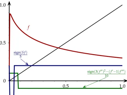
Figure 4.1: Panel A shows the graph of f(x) = 1920x(1−x)(5−4x+2x3). Ob- serve that condition(U)holds. Also note that f(f(x∗))> x∗ and condition(L) holds. Panel B shows, in the interval [α,β], the graphs of scaled versions of the sign function composed with, respectively, the Schwarzian derivative of f and 3(f′′)2−(f′−1)f′′′. Observe that the sign of 3(f′′)2−(f′−1)f′′′ remains positive, meanwhileS f changes sign in the interval[α,β].
247/320 ∈ (0, 1). Hence, f is well-defined. On the other hand, f′(x) = −1920(10x4−8x3− 12x2+18x−5) and so f′(0) = 194 > 1. Moreover, invoking again Sturm’s Theorem, f′ has exactly one real rootx∗ (which one can calculate explicitly since f′ is a polynomial of degree 4) in the interval (0, 1). At x∗ ≈ 0.3966 the function f attains a local maximum because f(0+) = f(1−) = 0. Solving the equation f(x) = x, we find that f has a unique solution K∈ (0, 1), which again can be explicitly calculated, withK ≈ 0.6441; and sox∗ < K. Thus, f satisfies the unimodal condition(U)with a = 0 and b= 1. Observe in Panel A in Figure4.1 that condition(L)holds for f becausex∗< α= f(f(x∗)).
Panel B in Figure4.1illustrates that Theorem1.1cannot be used to study the behaviour of equation (1.1) with f given by (4.1). Indeed, we observe that the condition(S)is violated, i.e.,
0 100 200 300 400 500 0
0.5 β¯
α¯
t
bbb
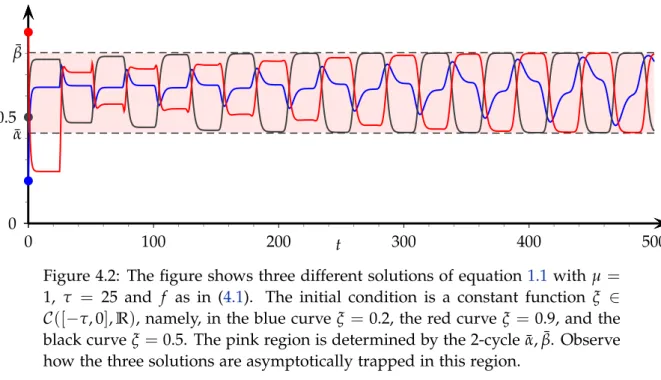
Figure 4.2: The figure shows three different solutions of equation1.1 with µ= 1, τ = 25 and f as in (4.1). The initial condition is a constant function ξ ∈ C([−τ, 0],R), namely, in the blue curveξ = 0.2, the red curveξ = 0.9, and the black curveξ =0.5. The pink region is determined by the 2-cycle ¯α, ¯β. Observe how the three solutions are asymptotically trapped in this region.
the Schwarzian derivative, S f, is not negative in the interval [α,β]. In contrast, the function 3(f′′)2−(f′−1)f′′′ has positive sign (again this is easily verified using Sturm’s Theorem in the interval [0, 1], which contains the interval [α,β]). Thus, f satisfies the assumptions of Theorem3.2.
Since f′(K)≈ −1.1390, invoking Theorem3.2we conclude that the sharpest invariant and attracting interval containing the attractor of equation (1.1) for all values of the delay τ is determined by the unique nontrivial 2-cycle{α, ¯¯ β}of f in the interval[α,β]. Numerically, we find that ¯α≈0.4269 and ¯β≈0.8013.
In Figure4.2, we plot three solutions of equation (1.1) with f as in (4.1),µ=1,τ=25 and different constant initial conditions. Observe that all the solutions asymptotically take values in the interval determined by the 2-cycle{α, ¯¯ β}as the result predicts. Moreover, observe that ast →∞the solutions oscillate in a range that it is close to the length of the interval[α, ¯¯ β]. ♢ The next example shows that Proposition 3.3 can be applied in situations where the as- sumptions in Theorem1.1, and in Theorem3.2, do not hold.
Example 4.2. Consider equation (1.1) with f: (0, 1)→(0, 1)given by f(x) = 3
10x (
1− 1 10ln(x)
)15
. (4.2)
Differentiating, we have f′(x) = 3
10 (
1− ln(x) 10
)15
− 9 20
(
1−ln(x) 10
)14
=−3(ln(x)−10)14(ln(x) +5)
1016 .
Therefore, f has a critical point atx∗ =e−5∈ (0, 1). Moreover, f′′(x) =−9(ln(x)−10)13(ln(x) +4)
2·1015x ,
0.5 1.0 0
0.5 1.0
f
sign(3(f′′)2−(f′−1)f′′′) 10
sign(S f) 5
Figure 4.3: Graphs of the function f(x) = 103x(1− 101 ln(x))15 (red curve), and the graphs of scaled versions of the sign function composed with, respectively, the Schwarzian derivative of f (blue curve) and 3(f′′)2−(f′ −1)f′′′ (green curve). Observe that at the fixed pointK,S f is positive and 3(f′′)2−(f′−1)f′′′
is negative. Sincex∗ ∈ [α,β], the assumptions of Theorem1.1 and Theorem3.2 are not satisfied.
and so f′′(x∗) < 0. Noting that f(0+) = 0 and f(1−) = 3/10, we conclude that f is well- defined and unimodal in the interval(0, 1). Now, note that f is convex in the interval(0, e−4) and limx→0+ f(x)/x = +∞. Consequently, f has a unique fixed pointK in the interval (0, 1) and it satisfiesx∗< K. This shows that(U)hold for (4.2)
Next, we obtain that
β= f(x∗) = 43046721e
−5
327680 ≈0.8852 , and
α= f(f(x∗)) = 129140163e
−5
3276800 (
1− 1 10ln
(43046721e−5 327680
))15
≈0.3185 .
Recalling that x∗ = e−5, we have that condition (L) holds. In this case, neither Theorem1.1 nor Theorem 3.2 can be used because the Schwarzian derivative and the function 3(f′′)2− (f′−1)f′′′ do not satisfy the sign restrictions in the interval[α,β], cf. Figure4.3.
Nevertheless, Proposition3.3holds. We need to verify that d(x) = f(x)
x = 3
10 (
1− 1 10ln(x)
)15
is decreasing, which is trivial, andg(x) =ln◦d◦exp satisfies 3(g′′)2−g′g′′′ >0 in the interval [lnα, lnβ]. Deriving, we obtain
3(g′′(x))2−g′(x)g′′′(x) = 225
(x−10)4, (4.3)
and 3(g′′(x))2−g′(x)g′′′(x)is positive in the interval[lnα, lnβ].
0 100 200 300 400 500 0
0.5 K
t
b
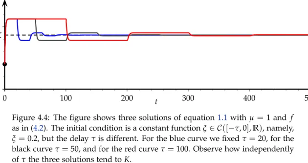
Figure 4.4: The figure shows three solutions of equation 1.1 with µ = 1 and f as in (4.2). The initial condition is a constant functionξ ∈ C([−τ, 0],R), namely, ξ =0.2, but the delayτis different. For the blue curve we fixedτ= 20, for the black curve τ=50, and for the red curveτ=100. Observe how independently of τthe three solutions tend toK.
Computing the derivative of f at its fixed pointK, we obtain that this derivative is greater than −1 (approx. −0.3843). By Proposition 3.3 for any initial condition ξ ∈ C([−τ, 0],(0, 1)) the solutions of (1.1) tend to K ast tends to +∞, with independence of the size of the delay τ>0 and the value of µ>0 as Figure4.4illustrates. ♢ Probably, the most famous representatives of equation (1.1) are the Nicholson’s blowflies equation and the Mackey–Glass equation. In the Nicholson’s blowflies equation f is given by
f(x) = 1
µxe−x, (4.4)
whereas in the Mackey–Glass equation f is given by f(x) = 1
µ ax
1+xb, a>0, b≥1. (4.5)
Both (4.4) and (4.5) have negative Schwarzian derivative, and therefore Theorem1.1can be used to study them. This was illustrated in [11, Section 3] with a couple of examples. We notice that Proposition3.3can be used to obtain the same conclusions as in those examples. Indeed, d(x) = f(x)/x is decreasing both for (4.4) and (4.5). Therefore, to invoke Proposition3.3 we need to check that g(x) = ln◦d◦exp satisfies 3(g′′)2−g′g′′′ > 0 in the interval (lnα, lnβ). The following examples show that the inequality holds not only in the interval(lnα, lnβ)but in the wholeR.
Example 4.3. Nicholson’s blowflies equation. In this case,g(x) =ln(1/µ)−ex and trivially 3(g′′)2−g′g′′′ =2e2x >0 . ♢ Example 4.4. The Mackey–Glass equation. In this case,g(x) =ln(a/µ)−ln(1+ebx)and after some straightforward calculations we obtain that
3(g′′)2(x)−g′(x)g′′′(x) = b
4e2bx(2+ebx)
(1+ebx)4 >0 . ♢
Acknowledgements
D. Franco and J. Perán were supported by grant MTM2017-85054-C2-2-P (AEI/FEDER, UE) and ETSII-UNED grant 2020-MAT10. D. Franco was supported by grant PRX19/00582 of the Ministerio de Educación, Cultura y Deporte (Subprograma Estatal de Movilidad). D. Franco thanks the Department of Mathematical Sciences of the University of Bath (UK) for its gener- ous hospitality during a sabbatical leave.
References
[1] S. Buedo-Fernández, E. Liz, On the stability properties of a delay differential neoclas- sical model of economic growth, Electron. J. Qual. Theory Differ. Equ.2018, No. 43, 1–14.
https://doi.org/10.14232/ejqtde.2018.1.43;MR3827981;Zbl 1413.34269
[2] E. Burger, On the stability of certain economic systems, Econometrica 24(1956), No. 4, 488–493.https://doi.org/10.2307/1905498;MR83410;Zbl 0072.37406
[3] W. A. Coppel, The solution of equations by iteration, Math. Proc. Cambridge 51(1955), No. 1, 41–43. https://doi.org/10.1017/S030500410002990X; MR100353;
Zbl 0064.12303
[4] D. Franco, J. Perán, J. Segura, Global stability of discrete dynamical systems via ex- ponent analysis: applications to harvesting population models, Electron. J. Qual. The- ory Differ. Equ. 2018, No. 101, 1–22. https://doi.org/10.14232/ejqtde.2018.1.101;
MR3896825;Zbl 1424.39038
[5] D. Franco, J. Perán, J. Segura, Stability for one-dimensional discrete dynamical systems revisited,Discrete Contin. Dyn. Syst. Ser. B25(2020), No. 2, 635–650.https://doi.org/10.
3934/dcdsb.2019258;MR4043583;Zbl 0715171753
[6] W. S. C. Gurney, S. P. Blythe, R. M. Nisbet, Nicholson’s blowflies revisited. Nature 287(1980), No. 5777, 17–21.https://doi.org/10.1038/287017a0
[7] A. F. Ivanov, A. N. Sharkovsky, Oscillations in singularly perturbed delay equations, in:
C. K. R. T. Jones, U. Kirchgraber, H.-O. Walther (eds.), Dynamics reported: expositions in dynamical systems, Dynam. Report. Expositions Dynam. Systems (N.S.), Vol. 1, pp. 164–
224. Springer, Berlin, Heidelberg, 1992. https://doi.org/10.1007/978-3-642-61243- 5_5;MR1153031;Zbl 0755.34065
[8] T. Krisztin, H.-O. Walther, Unique periodic orbits for delayed positive feedback and the global attractor, J. Dynam. Differential Equations 13(2001), No.1, 1–57. https://doi.
org/10.1023/A:1009091930589;MR1822211;Zbl 1008.34.061
[9] T. Krisztin, H.-O. Walther, J. Wu, Shape, smoothness and invariant stratification of an attracting set for delayed monotone positive feedback, Fields Institute Monographs, Vol. 11, American Mathematical Society, Providence, RI, 1999.MR1719128;Zbl 1004.34002 [10] B. Lani-Wayda, Erratic solutions of simple delay equations, Trans. Amer. Math. Soc.
351(1999), No. 3, 901–945.https://doi.org/10.1090/S0002-9947-99-02351-X;https:
//doi.org/www.jstor.org/stable/117910;MR1615995;Zbl 0943.34064
[11] E. Liz, G. Röst, On the global attractor of delay differential equations with unimodal feedback, Discrete Contin. Dyn. Syst. 24(2009), No. 4, 1215–1224. https://doi.org/10.
3934/dcds.2009.24.1215;MR2505701;Zbl 1188.32102
[12] M. C. Mackey, L. Glass, Oscillation and chaos in physiological control systems, Science 197(1977), No. 4300, 287–289. https://doi.org/10.1126/science.267326;
Zbl 1383.92036
[13] J. Mallet-Paret, R. D. Nussbaum, Global continuation and asymptotic behaviour for periodic solutions of a differential-delay equation, Ann. Mat. Pura Appl. (4) 145(1986), 33–128.https://doi.org/10.1007/BF01790539;MR886709;Zbl 0617.34071
[14] J. Mallet-Paret, R. D. Nussbaum, A differential-delay equation arising in optics and physiology, SIAM J. Math. Anal. 20(1989), No. 2, 249–292. https://doi.org/10.1137/
0520019;MR982660;Zbl 0676.34043
[15] J. Mallet-Paret, G. R. Sell, The Poincaré–Bendixson theorem for monotone cyclic feedback systems with delay, J. Differential Equations 125(1996), No. 2, 441–489. https:
//doi.org/10.1006/jdeq.1996.0037;MR1378763;Zbl 0849.34056
[16] G. Röst, J. Wu, Domain-decomposition method for the global dynamics of delay dif- ferential equations with unimodal feedback, Proc. R. Soc. Lond. Ser. A Math. Phys.
Eng. Sci. 463(2007), No. 2086, 2655–2669. https://doi.org/10.1098/rspa.2007.1890;
MR2352875;Zbl 1137.34038
[17] H. Smith, An introduction to delay differential equations with applications to the life sciences, Texts in Applied Mathematics, Vol. 57, Springer, New York, 2011.https://doi.org/10.
1007/978-1-4419-7646-8;MR2724792;Zbl 1227.34001
[18] H.-O. Walther, The 2-dimensional attractor ofx′(t) =−µx(t) + f(x(t−1)),Mem. Amer.
Math. Soc.113(1995), No. 544, 76 pp.https://doi.org/10.1090/memo/0544;MR1230775;
Zbl 0829.34063