A state-dependent delay equation with chaotic solutions
Benjamin B. Kennedy
B, Yiran Mao and Erik L. Wendt
Department of Mathematics, Gettysburg College, 300 N. Washington St, Gettysburg, PA, 17325, USA Received 2 November 2018, appeared 19 March 2019
Communicated by Hans-Otto Walther
Abstract. We exhibit a scalar-valued state-dependent delay differential equation x0(t) = f(x(t−d(xt)))
that has a chaotic solution. This equation has continuous (semi-strictly) monotonic negative feedback, and the quantityt−d(xt)is strictly increasing along solutions.
Keywords: differential delay equation, state-dependent delay, chaotic solution.
2010 Mathematics Subject Classification: 34K23.
1 Introduction
In this paper we consider the following differential delay equation with continuous monotonic negative feedback and state-dependent delay:
x0(t) = f(x(t−d(xt))). (1.1) Here “negative feedback” means that u f(u)<0 for all u6=0.
We shall writeC=C([−1, 0],R)for the space of continuous real-valued functions defined on [−1, 0], equipped with the sup norm. In the usual way, if I ⊆R is any interval containing [t−1,t]andx: I →Ris continuous, we writextfor the point inCdefined by
xt(s) =x(t+s), −1≤s ≤0,
and refer to xt as a segment of x. We shall take as the phase space for Equation (1.1) an appropriate subset X ⊆ C on which existence and uniqueness of solutions holds, and on which a continuous solution semiflow is defined. In particular, the delay functionald will be defined onXand will assume values between 0 and 1. By asolutionof Equation (1.1) we mean either a continuous functionx :[−1,∞)→Rsuch thatxt∈ Xfor allt≥0 and (1.1) holds for allt>0, or a continuous functionx:R→Rsuch thatxt∈ Xfor allt∈Rand (1.1) holds for allt∈R. In either case, we say thatxis thecontinuation of x0as a solution of Equation(1.1).
BCorresponding author. Email: bkennedy@gettysburg.edu
We are interested in the possibility of irregular or chaotic solutions of Equation (1.1) when Equation (1.1) has monotonic negative feedback. Our primary motivation is the impossibility of chaos in the “corresponding” constant-delay equation
x0(t) = f(x(t−1)). (1.2)
Suppose thatx : [−1,∞) → Ris a bounded solution of Equation (1.2), and writeω(x0) ⊆ C for the ω-limit set of x0. A version of the Poincaré–Bendixson theorem, due to Mallet-Paret and Sell [9] (and that actually has much wider applicability than we describe here), describes the structure ofω(x0)in the case that f is smooth and strictly monotonic with negative feed- back. On the “dynamical” side, Mallet-Paret and Sell’s Poincaré–Bendixson theorem states thatω(x0)must be either a single non-constant periodic orbit, or must consist of the equilib- rium point{0}and (perhaps) solutions homoclinic to{0}(though solutions homoclinic to{0} seem unlikely to exist, and results in [8] imply that they cannot exist if{0}is hyperbolic). On the “geometric” side, the theorem states that the mapΠ:ω(x0)→R2 given by the formula
ω(x0)3 ϕ7→Π(ϕ) = (ϕ(0),ϕ(−1))∈R2
is injective. This injectivity has the consequence that, ifz0 <z1 <z2are three successive zeros of a nontrivial periodic solution p, then p has minimal period z2−z0 – loosely speaking, p has “one oscillation about zero per minimal period.”
It is known already that the state-dependent delay in Equation (1.1) allows for substantial changes in the dynamics of solutions. In [4], for example, an instance of Equation (1.1) is devised for which f is smooth and strictly decreasing and that has a periodic solution p for which the above-described mapΠis not injective on{pt}= ω(p0). The papers [7], [13], [14], and [15] describe a state-dependent delay equation
x0(t) =−αx(t−d(xt)), α>0
with negative feedback and for which{0}is hyperbolic, but that nevertheless has a solution homoclinic to{0}and chaotic solutions near this homoclinic solution.
In the present paper, we wish to restrict attention to cases of Equation (1.1) where the delay functional is, in some (subjective) sense, not too dissimilar to the constant delay case.
In particular, we are interested in cases where the delayd(xt)is strictly positive but bounded, and where the delayed timet−d(xt)is strictly increasing with respect totfor any solutionx.
We shall abbreviate this latter condition as (DTI). More specifically, condition (DTI) is defined as follows, wherex:[−1,∞)→Ris a solution of Equation (1.1):
t+e−d(xt+e)>t−d(xt) for anyt ≥0 and anye>0. (DTI) Condition (DTI) (or close analogs) has been used by many authors in the study of state- dependent delay equations. On the conceptual side, (DTI) means that states influence the feedback response in the expected temporal order (though for a discussion of the delayed time t−d(xt)beingmonotonicbut not necessarily increasing see [12]); on the analytical side, (DTI) facilitates the by-now-familiar organization of the phase space according to a non-increasing
“oscillation speed.” (In the above-mentioned papers [7], [13], [14], and [15], the “oscillation speed” of the solution homoclinic to{0}increases, and condition (DTI) does not hold; condi- tion (DTI) does hold for the equation considered in [4].)
Here, then, is the main theorem for the paper.
Theorem 1.1. There is an instance of Equation(1.1)for which the following hold.
(i) f is continuous, non-increasing, and satisfies the negative feedback condition.
(ii) A continuous solution semiflow for Equation (1.1) is defined on a subset X ⊆ C of bounded functions with bounded Lipschitz constant.
(iii) (DTI)holds for all solutions of Equation(1.1)with segments in X.
(iv) Given any k∈ N, there is a periodic solution pk of Equation(1.1)such that pkt ∈X for all t∈R and such that the interval [0,ρ] contains precisely 2k+1 zeros of pk, where ρ is the minimal period of pk.
(v) There is a solution v of Equation(1.1)such that vt ∈ X for all t∈ Rand such that, given any k ∈N, there is a sequence tn→∞such that vtn → pk0.
Point (iv) demonstrates the violation of the “geometric” part of Mallet-Paret and Sell’s Poincaré–Bendixson theorem; point (v) demonstrates the violation of the “dynamic” part.
Points (iv) and (v) together constitute what we mean by our particular instance of Equation (1.1) being “chaotic”. As we proceed, however, we shall see that it is possible to specify the version of Equation (1.1) described in Theorem1.1so that the following is also true: there is a subset M ⊆ X, a return mapR: M → Mfor Equation (1.1), an interval I ⊆ [0, 1], and a map h:R→I such that
• the restricted dynamical systemh2: I → I is semiconjugate to R: M →M; and
• there is a subinterval of I on whichh2 is chaotic (in the sense of Devaney).
This is another sense in which our example equation can be considered to be “chaotic.”
Remark 1.2. Chaotic solutions in the constant-delay case (Equation (1.2)) are known to be possible in the case that f is non-monotonic with negative feedback (see, for example, [10]
and [11], or [5] and [6]).
Remark 1.3. While Theorem1.1illustrates how variable delay can complicate solution behav- ior, we emphasize that the feedback function f in Theorem1.1 is only nonincreasing, rather than strictly decreasing; accordingly, Theorem 1.1, by itself, does not quite illustrate that the Poincaré-Bendixson theorem fails merely by the introduction of state-dependent delay.
The paper is organized as follows. In Section 2 we give a very simple existence and uniqueness result that is adequate for our purposes. In Section 3 we define our particular equation of interest. In Section 4 we make the explicit estimates that we need, and prove Theorem1.1.
2 Existence and uniqueness
Throughout, if AandBare metric spaces with metricsdAanddB, respectively, andH: A→B is any function, we write`(H)for the global Lipschitz constant forH, provided that it exists:
`(H) = sup
a16=a2
dB(H(a1),H(a2)) dA(a1,a2) .
As stated above, we write C = C([−1, 0],R), equipped with the sup norm. Throughout we write
X={ϕ∈C : kϕk ≤1, `(ϕ)≤1}. By the Ascoli–Arzelà Theorem,Xis a compact subset ofC.
We shall assume throughout that f :R→Rsatisfies the following hypotheses:
(f is nonincreasing, f is Lipschitz (i.e. `(f)< ∞), andu f(u)<0 for allu6=0;
|f(u)| ≤1 for allu∈R. (Hf)
We shall assume throughout thatd: X→Rsatisfies the following hypotheses:
0<dmin ≤d(ϕ)≤dmax≤1 for all ϕ∈X;
dis Lipschitz (i.e. `(d)<∞);
There is someα∈ (0, 1)such that, ifϕ∈Xandψ∈Xand ϕ(s) =ψ(s)for alls ∈[−1,−α], thend(ϕ) =d(ψ).
(Hd)
The assumptions on the range ofd and thatd is Lipschitz are familiar; the final assumption says that d(ϕ) depends only on the restriction of ϕ to [−1,−α] and substantially simplifies our work both in this section and later.
Here is the existence and uniqueness theorem that we shall use. The ideas are, by now, standard.
Proposition 2.1. Assume that f : R → R satisfies Hypotheses (Hf) and that d : X → R satisfies Hypotheses(Hd). Then Equation(1.1)has a uniquely defined continuous solution semiflow F:R+× X→X.
Proof. Choose and fix β∈(0, min(dmin,α)), wheredmin andαare as in (Hd).
Given ϕ ∈ X, let ˜x : [−1,β] → R be any extension of ϕto [−1,β]with |x˜(s)| ≤ 1 for all s∈[−1,β]and`(x˜)≤1 – otherwise put, ˜xs∈Xfor alls ∈[0,β](we may, in particular, take ˜x to be constant on[0,β]). Observe that the function
[0,β]3s 7→x˜(s−d(x˜s))
is continuous and does not depend on the particular extension ˜x of ϕ. Definex: [−1,β]→R by the formula
x0= ϕ; x(t) =x(0) +
Z t
0 f(x˜(s−d(x˜s)))ds, s ∈[0,β]. Observe that, fort ∈(0,β),
|x0(t)|=|f(x˜(s−d(x˜s)))| ≤1, and so`(x)≤1.
Imagine (for example) thatx(t)>1 for somet ∈ (0,β). By the mean value theorem there must be somet0 ∈ (0,t) with x(t0) > 1 and x0(t0) > 0. Since `(x) ≤ 1, however, we must havex(s) > 0 for all s ∈ [t0−1,t0]; in particular, ˜x(t0−d(x˜t0)) = x(t0−d(x˜t0)) > 0 and so x0(t0) = f(x˜(t0−d(x˜t0))) < 0, a contradiction. We conclude that x(t) ≤ 1 for all t ∈ [0,β]; the proof thatx(t)≥ −1 for allt ∈ [0,β]is similar. Thus we see that xt ∈ X for allt ∈ [0,β], and so conclude thatd(xt)is defined and, by (Hd), equal to d(x˜t)for allt ∈ [0,β]. It follows
that x solves Equation (1.1) fort ∈ (0,β). Moreover, if y : [−1,β] → R is continuous, solves Equation (1.1) fort ∈ (0,β), and satisfies y0 = ϕ, from (Hd) we see thaty0(t) = x0(t)for all t ∈ (0,β); thus x is theunique solution of Equation (1.1) on [−1,β] with x0 = ϕ. Continuing forward by steps establishes the existence of the solution semiflow F:R+×X→X.
Suppose that ϕ,ψ ∈ X have continuations x and y, respectively, as solutions of Equation (1.1). Write ˜ϕ and ˜ψ for extensions of ϕand ψ, respectively, to [−1,∞) that are constant on [0,∞). Observe that for anyt∈[0,β], whereβis as above, by (Hd) we haved(xt) =d(ϕ˜t)and d(yt) =d(ψ˜t); we also of course havekϕ˜t−ψ˜tk ≤ kϕ−ψk. Thus fort∈ [0,β]we have
|d(xt)−d(yt)|= |d(ϕ˜t)−d(ψ˜t)| ≤`(d)kϕ−ψk, and so (using the fact that `(y)≤1) we have, fort ∈[0,β], that
|x0(t)−y0(t)|=|f(x(t−d(xt)))− f(y(t−d(yt)))|
≤`(f)h|x(t−d(xt))−y(t−d(xt))|+|y(t−d(xt))−y(t−d(yt))|i
≤`(f)hkϕ−ψk+`(d)kϕ−ψki=`(f)(1+`(d))kϕ−ψk. Thus, fort ∈[0,β]we have
|x(t)−y(t)| ≤[1+β`(f)(1+`(d))]kϕ−ψk=:mkϕ−ψk. Therefore, given any t, ¯t ≥0, assumingt∈[kβ,(k+1)β)we have
|x(t)−y(¯t)| ≤ |x(t)−y(t)|+|y(t)−y(t¯)| ≤mk+1kϕ−ψk+|t−t¯|. The continuity of the solution semiflow follows.
Remark 2.2. The hypotheses of Proposition 2.1 are not sufficient for (DTI) to hold. It is not hard to see that certain additional assumptions ond(for example, that`(d)<1) are enough to guarantee (DTI); below, our verification that (DTI) holds for our particular equation of interest is somewhat more involved.
3 A particular instance of Equation (1.1)
We begin by specifying our feedback function f as follows: whereη>0,
f(u) =
1, u≤ −η;
−u/η, u∈[−η,η];
−1, u≥η.
(We shall impose additional conditions on η later.) The function f is pictured in Figure3.1.
Note that f is nonincreasing, that f has negative feedback and Lipschitz constant η−1, and that |f(u)| ≤1 for all u ∈ R– that is, that f satisfies Hypotheses (Hf). We henceforth take f andηas described above.
We now turn to the definition of our delay functional d. We shall need the following lemma.
Lemma 3.1. Let 0 < a < b ≤ 1 be given. There is a Lipschitz map g : R → [a,b] that satisfies
`(g)≤2and that has the following properties:
(i) Given any k∈ N, the discrete dynamical system g2: [a,b]→[a,b]has a periodic pointq˜k that has minimal period k.
(ii) There is a point q˜ ∈[a,b]such that, given any k ∈ N, there is a strictly increasing sequence nj
of natural numbers such that g2nj(q˜)→q˜kas j→∞.
Proof. First letG :R → [0, 1]be any map with `(G)≤ 2 and for which there is a subinterval S⊆[0, 1]such that
• G2(S)⊆S;
• For each k ∈ N, the subintervalS contains a periodic point of minimal periodk of the restricted discrete dynamical systemG2 :[0, 1]→[0, 1];
• The restricted discrete dynamical system G2 : [0, 1] → [0, 1] has an orbit that is dense inS.
Examples of such mapsGare well-known; see Remark3.3 below.
Now given 0<a <b≤1, we defineg :R→[a,b]by the formula g(x) =a+ (b−a)G
x−a b−a
. Observe that`(g) =`(G).
The restricted discrete dynamical system g : [a,b] → [a,b] is conjugate to the restricted discrete dynamical systemG : [0, 1] → [0, 1](via the conjugacy H(x) = (b−a)x+a), and so likewise g2 : [a,b] →[a,b]is conjugate to G2 : [0, 1]→ [0, 1]. Thus g2, analogously to G2, has a forward-invariant interval ˜S⊆[a,b]that contains periodic points of every possible minimal period and a dense orbit. Any point in this dense orbit satisfies point (ii) of the lemma.
−1.0 −0.5 0.0 0.5 1.0
−1.0−0.50.00.51.0
u
f(u) − η η
Figure 3.1: The feedback function f. We shall henceforth writeg,aandbas in Lemma3.1.
As we proceed, we shall also need the function described in the following lemma, which is slightly different fromg.
Lemma 3.2. Let a, b, and g be as Lemma 3.1, and let c ∈ R. The function h : R → [a−c,b−c] given by
h(u) =g(u+c)−c for all u∈[a−c,b−c] has the following properties:
(i) Given any k ∈ N, the discrete dynamical system h2 : [a−c,b−c] → [a−c,b−c] has a periodic point qk that has minimal period k.
(ii) There is a point q ∈ [a−c,b−c] such that, given any k ∈ N, there is a strictly increasing sequence njof natural numbers such that h2nj(q)→qk as j→∞.
Proof. The lemma follows from the fact thathis conjugate to g.
Remark 3.3. There are many maps G : R → [0, 1] satisfying the conditions in the proof of Lemma3.1. For example, the so-calledTent Map T:R→[0, 1]is given by
T(u) =
0,u≤0;
2u,u∈[0, 1/2]; 2−2u,u∈[1/2, 1]; 0,u≥1.
T2 is well-known to have periodic points of all minimal periods and an orbit that is dense in [0, 1]; moreover, the restricted map T2 : [0, 1] → [0, 1]is chaotic in the sense of Devaney (see, for example, [1] or [3] for further discussion of this idea).
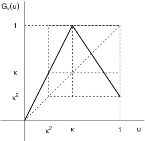
Here we introduce another class of such maps, primarily because it is these maps we use in our numerical examples below. Let κ ∈ (0, 1), and consider the function Gκ : R → [0, 1] given by
Gκ(u) =
0,u≤0;
u
κ, u∈ [0,κ];
1−(u−κ)(1+κ), u∈[κ, 1]; κ2, u≥1.
Observe thatGκ has slope 1/κon [0,κ]and slope−(1+κ)on[κ, 1]. Therefore
`(Gκ) =max
1 κ, 1+κ
and`(Gκ)≤2 as long asκ ∈[1/2, 1]. (The minimum value for`(Gκ)is attained atκ= −1+
√5
2 ,
where
`(Gκ) = 1
κ =1+κ= 1+√ 5 2 .)
Graphs ofGκ andGκ2are shown in Figures3.2and3.3, respectively.
Write
A1= [κ2,κ], A2=
κ,1+κ2 1+κ
, and A3=
1+κ2 1+κ, 1
. As is clear from the figure and readily verified with direct computation,
G2κ(A1) = A1∪A2∪A3, G2κ(A2) = A1∪A2∪A3, and Gκ2(A3) =A2∪A3.
1 1
κ2 κ2
κ κ
Gκ(u)
u
Figure 3.2: The function Gκ.
1 1
κ2 κ2
κ κ
G2
κ(u)
u 1+ κ2
1+ κ 1+ κ2
1+ κ
Figure 3.3: The functionGκ2.
Using familiar ideas (see, for example, [2]) one can now show that the restricted dynamical systemGκ2: A1∪A2∪A3→ A1∪A2∪A3 is semiconjugate to a chaotic subshift of finite type on three symbols, has periodic points of all minimal periods, and has a dense orbit (and is chaotic in the sense of Devaney).
We now define our delay functionaldon Xin several steps, showing that conditions (Hd) and (DTI) hold.
Chooseα∈ (0, 1). First, given ϕ∈ X, we write µ(ϕ) = max
s∈[−1,−α]|ϕ(s)|.
Lemma 3.4. The functionalµ: X→Rsatisfies `(µ)≤1.
Proof. Let ϕ,ψ∈ Xbe given. Suppose that
s∈[−max1,−α]|ϕ(s)|
is attained at the pointt1 and that
max
s∈[−1,−α]
|ψ(s)|
is attained at the pointt2. Then
µ(ψ)≥ |ψ(t1)| ≥ |ϕ(t1)| − kψ−ϕk=µ(ϕ)− kψ−ϕk and
µ(ϕ)≥ |ϕ(t2)| ≥ |ψ(t2)| − kψ−ϕk= µ(ψ)− kψ−ϕk, which yields
kψ−ϕk ≥µ(ϕ)−µ(ψ) and kψ−ϕk ≥µ(ψ)−µ(ϕ) and so
|µ(ψ)−µ(ϕ)| ≤ kψ−ϕk – that is,`(µ)≤1.
Withαandµas above, we now define the functionalν: X→Rby ν(ϕ) =minn
µ(ϕ)− |ϕ(−1)|,µ(ϕ)− |ϕ(−α)|o.
Remark 3.5. Observe thatν(ϕ) =0 precisely when the maximum of|ϕ(s)|s∈[−1,−α] is attained at either−1 or at−α. One consequence of this observation is the following. Ifx :[−1,∞)→R is a function with xt ∈Xfor all t≥0 andν(xt)6=0 for all t∈(t0,t1)⊆[0,∞), then
max{|xt(s)|:s∈[−1,−α]}
is never attained at s = −1 or at s = −α as t runs over (t0,t1). It follows that t 7→ µ(xt) is constant on(t0,t1)and therefore, by continuity, constant on[t0,t1]. Otherwise put,if(t0,t1)is any interval where the function t 7→ν(xt)is nonzero, the map t7→ µ(xt)is constant on[t0,t1].
The following lemma is elementary and we omit the proof.
Lemma 3.6.
(1) Suppose that Y is a metric space and that h1 : Y → R+ and h2 : Y → R+ are two Lipschitz functions. Then the function defined by
h(y) =min(h1(y),h2(y)) is Lipschitz with`(h)≤max(`(h1),`(h2)).
(2) Suppose that W, Y, and Z are metric spaces and that h1 :W →Y and h2:Y→Z are Lipschitz functions. Then h2◦h1is Lipschitz with
`(h2◦h1)≤`(h2)×`(h1).
(3) Suppose that Y is a compact metric space and that h1 : Y → R+ and h2 : Y → R+ are two Lipschitz functions. Then the function h:Y →R+defined by
h(y) =h1(y)×h2(y) is Lipschitz with
`(h)≤max
Y |h1(y)|`(h2) +max
Y |h2(y)|`(h1). Lemma 3.7. `(ν)≤2.
Proof. Consider the map defined by
ν∗(ϕ) =µ(ϕ)− |ϕ(−1)|.
Given ϕ,ψ∈ X, by Lemma3.4and the triangle inequality we have
|ν∗(ϕ)−ν∗(ψ)|=µ(ϕ)−µ(ψ) +|ψ(−1)| − |ϕ(−1)| ≤µ(ϕ)−µ(ψ)+|ψ(−1)| − |ϕ(−1)|
≤2kϕ−ψk.
Thus`(ν∗)≤2. A similar argument shows that the map ν∗(ϕ) =µ(ϕ)− |ϕ(−α)|
also has Lipschitz constant no more than 2. The lemma now follows from the first part of Lemma3.6.
Givenγ0 ∈(0, 1)and 0<c1 <c2<∞, we now defineγ:(0,∞)→(0,∞)as follows:
γ(u) =
γ0, u∈[0,c1]; γ0+ c1−γ0
2−c1(u−c1), u∈ [c1,c2]; 1, u≥c2.
That is, γ is constant on [0,c1]; linear on [c1,c2]; and equal to 1 on [c2,∞). Observe that
`(γ) = c1−γ0
2−c1.
Now let η be as in the definition of f at the beginning of Section 3. Let g be as in the statement of Lemma3.1. Remember in particular thatg is Lipschitz with`(g)≤2 and that g maps Rinto [a,b] ⊆ (0, 1](we shall specify the constants a andb later). We now define our delay functionald: X→Ras follows:
d(ϕ) =γ(ν(ϕ))g(µ(ϕ) +η/2). (D) We shall taked as defined in (D) henceforth.
Lemma 3.8. The functional d: X→R+defined in(D)is Lipschitz.
Proof. The lemma follows from the fact thatµ,ν,γandg are Lipschitz, and from Lemma3.6.
Observe that this delay functional d satisfies the hypotheses (Hd): d(ϕ) is bounded be- tween γ0a>0 andb≤1 for all ϕ, and depends only on the restriction of ϕto[−1,−α].
Let us now consider whether (DTI) holds for solutions of Equation (1.1) with segments in X, when the delay functional d is as defined in (D). Suppose that x : [−1,∞) → R is a function with xt ∈ Xfor all t ≥0. We now show that, under appropriate assumptions on the parametersa,b,γ0,c1andc2,
t+e−d(xt+e)>t−d(xt)
for allt ≥0 ande>0. Since f anddsatisfy the conditions given in Proposition2.1, it follows that (DTI) holds for solutions of Equation (1.1) with segments in X.
Lemma 3.9. Suppose that x:[−1,∞)→Rsatisfies xt∈ X for all t≥0. For any t≥0ande>0,
|ν(xt+e)−ν(xt)| ≤e.
(Thus, while the functionalνdoes not satisfy`(ν)≤1, the function s 7→ν(xs)
does have Lipschitz constant no greater than 1.)
Proof. The functions7→ν(xs)is continuous; thus the set S= {s∈[t,t+e] : ν(xs) =0} is closed.
Case 1: if Sis empty then, by our observation in Remark3.5,µ(xs)is equal to some constant ξ fors ∈[t,t+e]. Thus, forsin this range,ν(xs)can be written
ν(xs) =minn
ξ− |x(s−1)|,ξ− |x(s−α)|o,
and in this case the map s7→ ν(xs)is clearly Lipschitz on[t,t+e]with Lipschitz constant no greater than 1 (recall part 1 of Lemma3.6).
Case 2: ifSis nonempty, write
t+e1=sup{s∈ [t,t+e] : s∈S}.
ν(xt+e1) = 0 sinceSis closed. Ift+e1 = t+e, then obviouslyν(xt+e1) = ν(xt+e); ift+e1 <
t+e, thenν(xs) is nonzero fors ∈ (t+e1,t+e)and an argument like that in Case 1 shows that the map s 7→ ν(xs) has Lipschitz constant no more than 1 on [t+e1,t+e]. Whether t+e1 =t+eor not, then, we have
|ν(xt+e)−ν(xt+e1)| ≤e−e1.
But since ν(xt+e1) =0 andνis nonnegative, this last estimate tells us that ν(xt+e)∈[0,e−e1].
Now, if ν(xt) =0, we’re done. Otherwise, set
t+e0 =inf{s∈[t,t+e] : s ∈S}.
Then sinces7→ν(xs)is nonzero on(t,t+e0), another argument like that in Case 1 shows that s7→ ν(xs)has Lipschitz constant no more than 1 on [t,t+e0]and so (sinceν(xt+e0) =0) that ν(xt)∈[0,e0]. Thus (recalling thate0≤e1) we obtain
|ν(xt+e)−ν(xt))| ≤e0+e−e1≤e, as desired.
With x, t and e as in the statement of Lemma 3.9 just above, let us now consider the quantity d(xt+e)−d(xt). Since s 7→ ν(xs) has a Lipschitz constant no more than one on [t,t+e], we can find a finite set of points
t=s0< s1 <· · ·<sm =t+e
such that, givenj∈ {1, . . . ,m},ν(xs)is either in the interval[0,c1]for alls ∈[sj−1,sj]or in the interval[c1/2,∞)for alls∈ [sj−1,sj]. In the former case,γ(ν(xs))is equal toγ(0) =γ0on the subintervals ∈ [sj−1,sj]and so the Lipschitz constant of s 7→ d(xs) on this subinterval is no more than
γ0×`(g)×`(µ)×`(s7→ xs), which by the definition ofXand Lemma3.4is no more than
γ0`(g).
In the latter case,µ(xs)is constant on the subintervals∈ [sj−1,sj]and so the Lipschitz constant ofs7→ d(xs)on the subinterval is no more than`(γ)×`(s7→ν(xs))×b=`(γ)×b.
These estimates establish the following proposition.
Proposition 3.10. Assume that d is such that
`(γ)b= 1−γ0
c2−c1b<1 and γ0`(g)<1.
Then, if x:[−1,∞)→Ris any function with xt ∈X for all t ≥0, we have t+e−d(xt+e)>t−d(xt)
for any t≥ 0 and anye > 0. In particular, since d and f satisfy(Hd) and(Hf), respectively, (DTI) holds along all solutions of Equation(1.1)with segments in X.
We shall henceforth consider Equation (1.1) withdand f as defined in this section.
4 The set M and the map R
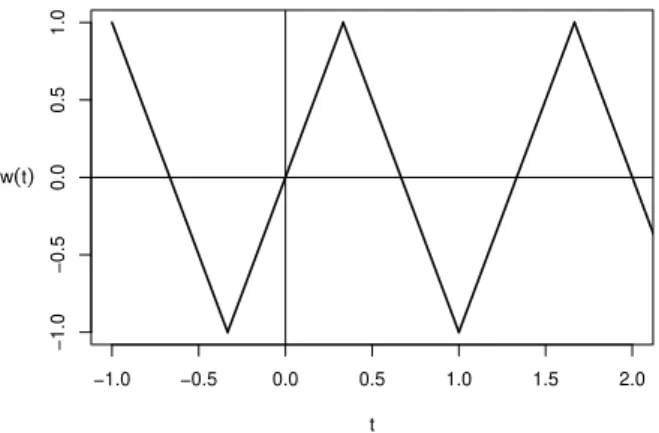
The construction that follows is motivated by the following observation. The constant-delay equation
y0(t) =−sign(y(t−1/3))
has a periodic solutionw whose zeros are separated by 2/3 and that satisfiesw(0) = 0 and w0(0) =1. This solution is pictured in Figure4.1.
The solutions of Equation (1.1) that we will construct are “close” to the solutionw.
We define the functionalλ: X→Ras follows:
λ(ϕ) =max{|ϕ(s)| :s∈ [−2/3, 0]}.
The following Lemma is proven very much like Lemma3.4; accordingly, we omit the proof.
−1.0 −0.5 0.0 0.5 1.0 1.5 2.0
−1.0−0.50.00.51.0
t w(t)
Figure 4.1: The solution w.
Lemma 4.1. `(λ)≤1.
For the reader’s convenience we recall the following notation and parameters.
• η>0 – the feedback function f is linear on[−η,η], and f(u) =−sign(u)foru∈/[−η,η].
• `(g)– the Lipschitz constant of g.
• 0< a<b≤1 – the functiongmapsRto[a,b].
• α ∈ (0, 1) – µ(ϕ) and ν(ϕ)(and hence d(ϕ)) are determined by the restriction of ϕto [−1,−α].
• 0 <c1 < c2, andγ0 ∈ (0, 1)– the functionγis equal toγ0 on [0,c1], is linear on[c1,c2], and is equal to 1 on[c2,∞).
Recall also our formula ford:
d(ϕ) =γ(ν(ϕ))g(µ(ϕ) +η/2).
We shall henceforth set and fixα=1/3. We impose the following additional requirements on our parameters:
(i) γ0`(g)<1.
(ii) b(1−γ0)/(c2−c1)<1.
(iii) η< γ0a.
(iv) 6η<1/3.
(v) 1/3−η≤ a<b≤1/3+η.
(vi) 1/3−6η>c2.
Conditions (i) and (ii) are just the conditions given in Proposition 3.10for (DTI) to hold.
We shall need the other conditions below. The following particular choice of values shows that conditions (i)–(vi) can be satisfied.
η=1/100;
`(g) =2;
a =1/3−ηandb=1/3+η;
γ0 =9/20;
c2 =1/4;
c1 =1/100.
(C)
We now define the following subset M ⊆X.
M =
ϕ∈ X :
(I)ϕ(0) =0;
(II)ϕ0(s) =1 for alls ∈(−η, 0); (III)|ϕ(−2/3)| ≤2η;
(IV)ϕ(s)≤ −ηfor alls∈[−2/3+3η,−η]; (V)λ(ϕ)≥1/3−2η
.
A typical element ϕ of M is pictured in Figure 4.2. The size of η is exaggerated in the figure.
t ϕ(t)
−1 −2 3
− η
Figure 4.2: An element ϕof M.
There are two piecewise linear elements ψ1 and ψ2 of M with the following properties.
ψ1has
• slope 1 on[−1/3+2η, 0];
• slope 0 on[−1/3−2η,−1/3+2η];
• slope −1 on [−1,−1/3−2η]. ψ2has
• slope 1 on[−1/3−η, 0];
• slope −1 on [−1,−1/3−η].
These two points of Mmake it easy to see the following lemma, whose proof we omit.
Lemma 4.2. [1/3−2η, 1/3+η]⊆λ(M).
Assume thatϕ=x0∈ Mhas continuationx: [−1,∞)→Ras a solution of Equation (1.1).
We now studyx.
Proposition 4.3. Assume that points (i)–(vi) above hold, and that ϕ= x0 ∈ M has continuation x as a solution of Equation(1.1). Then x has a first positive zero z, and the following hold:
(a) z=2g(λ(ϕ) +η/2);
(b) −xz ∈ M, withλ(−xz) =g(λ(ϕ) +η/2)−η/2;
(c) if y0 ∈ M has continuation y as a solution of Equation(1.1)andλ(y0) = λ(x0), then y|[0,z] = x|[0,z].
Observe that point (b) says thatλ(ϕ)(and the fact thatϕ∈ M)determines λ(−xz). More- over, point (c) says that λ(ϕ)(and the fact that ϕ ∈ M) completely determines the restriction of x to[0,z]. Proceeding inductively, we see thatλ(ϕ)determines all of x|[0,∞). Moreover, we shall see that the sequence of (absolute values) of local extrema of x is an orbit of a discrete dynamical system determined by a functionhas in Lemma3.2. The properties of solutions of Equation (1.1) described in Theorem1.1 follow from corresponding properties of h2; the rest of the paper amounts to a detailed explanation of this idea.
We now prove Proposition4.3.
Proof. Observe first that, by points (iii), (iv), and (v),
d(x0)∈[γ0a,b]⊆ (η, 1/3+η]⊆(η, 2/3−3η),
and so in particular −d(x0)∈(−2/3+3η,−η)and (by (IV))x(−d(x0))≤ −η.
Now let us consider the interval [1/3−2η, 1/3+2η]. As t runs over this interval, t−1 runs over the interval [−2/3−2η,−2/3+2η]. Since |x(−2/3)| ≤ 2η (by (III)) and x has Lipschitz constant 1, we see that |x(t−1)| ≤4ηastruns over[1/3−2η, 1/3+2η]. Similarly,
|x(t−1/3)| ≤ 2ηas t runs over [1/3−2η, 1/3+2η]. We can draw three conclusions. First, since λ(ϕ)≥1/3−2η >4η (by (iv) and (V)), max{|ϕ(s)|: s∈ [−2/3, 0]}is actually attained at some s ∈ [−2/3+2η,−2η]. Second and similarly, µ(xt) is constant (and equal to λ(ϕ)) across allt ∈[1/3−2η, 1/3+2η]. Finally, astruns across[1/3−2η, 1/3+2η], since
µ(xt)− |x(t−1)| ≥1/3−2η−4η=1/3−6η> c2 and
µ(xt)− |x(t−1/3)| ≥1/3−2η−2η=1/3−4η>c2
(by (vi)) we have that γ(ν(xt)) = 1 for all such t. We conclude that as t runs over the interval [1/3−2η, 1/3+2η], d(xt)is constantand is equal to
g(λ(ϕ) +η/2) =:d∗.
See Figure4.3. The solution xis in black, and the value ofd(xt)is in blue.
Now, since [a,b] ⊆ [1/3−η, 1/3+η], d∗ ∈ [1/3−η, 1/3+η]. As t traverses the in- terval [1/3−2η, 1/3+2η], t−d∗ traverses an interval that contains the interval [−η,η]; more particularly, t−d∗ will traverse the interval [−η,η] precisely as t traverses the interval [d∗−η,d∗+η] ⊆ [1/3−2η, 1/3+2η]. Since−d(x0) ≥ −2/3+3η, d∗−η−d(xd∗−η) = −η, and (DTI) holds, we actually can now conclude that t−d(xt) ∈ [−2/3+3η,−η] for all t ∈ [0,d∗−η], and hence (by (IV)) that x0(t) = 1 for all t ∈ [0,d∗−η]. Thus, in particu- lar, x(d∗−η) =d∗−η≥1/3−2ηandx(−η+s) =−η+sfor all s∈[0, 2η].
−1.0 −0.5 0.0 0.5
−0.20.00.2
TIME
1 3−2η 1 3+2η
d*
z
Figure 4.3: The solution xand the functiont7→ d(xt).
On[d∗−η,d∗+η], then,x solves the ODE
x(d∗−η) =d∗−η, x0(d∗−η+s) = f(−η+s) =1−s/ηfor alls∈ [0, 2η]. Direct computation shows that, fors∈ [0, 2η], we have
x(d∗−η+s) =d∗−η+s− s
2
2η and so in particular
x(d∗) =d∗−η/2
– this is the maximum value ofxon [d∗−η,d∗+η]. x will traverse a symmetric arc astruns over[d∗−η,d∗+η]; we have x(d∗+η) =d∗−ηandx0(d∗+η) =−1.
Since (DTI) holds, we will have x0(t) = −1 at least from time t = d∗+ηuntil such time ast−d(xt) > ηand x(t−d(xt)) = η. Before this can occur, since η is less than the smallest possible delay (by (iii)), xwill attain a first zeroz =2d∗. This completes the proof of part (a) of the proposition. Part (c) is also clear:λ(ϕ)(and the fact thatϕ∈ M) completely determines the restriction ofxto [0,z].
It remains to check part b). We certainly have xz(0) = 0, and, since z = 2d∗ ≥ 2/3− 2η > 1/3+3η ≥ d∗+2η, we certainly have that x0z(s) = −1 for all s ∈ [−η, 0]. z−2/3 is in the interval [−2η, 2η]. Since x(0) = 0 and x has Lipschitz constant 1, we certainly have that |xz(−2/3)| ≤ 2η, as desired. Similarly, z−2/3+3η ≥ η, so xz(s) ≥ η for all s ∈ [−2/3+3η,−η]. Finally, since x(d∗) = d∗−η/2 > 2η, the maximum of |x(t)| as t runs over[z−2/3,z] is clearly attained atd∗, and x(d∗) ≥ 1/3−η−η/2 ≥ 1/3−2η. Thus
−xz ∈ M, as desired; and it is clear thatλ(−xz) =d∗−η/2= g(λ(ϕ) +η/2)−η/2.
Since d is even and f is odd, similar considerations let us see that x will have an infinite sequence of simple positive zerosz=z1< z2 <z3 <· · · with
(−1)nxzn ∈ M for alln∈N.
We have the following formulas:
λ(−xz1) =g(λ(x0) +η/2)−η/2;
λ(xz2) =g(λ(−xz1) +η/2)−η/2=g2(λ(x0) +η/2)−η/2;
λ(−xz3) =g(λ(xz2) +η/2)−η/2= g3(λ(x0) +η/2)−η/2;
...
λ((−1)nxzn) =gn(λ(x0) +η/2)−η/2;
...
Let us define the mapR : M → M by the formula R(x0) = xz2. Sincez2 > 4/3−4η > 1 for any x0 ∈ M, we observe that
(∗∗) λ(x0)completely determinesR(x0). We also have the following lemma.
Lemma 4.4. R: M→ M is Lipschitz continuous.
Proof. Our work so far shows that the mapZ :x0 7→ z2 is bounded by 4/3+4η, and is Lips- chitz becauseλand gare Lipschitz. Thus the kind of estimate in the proof of Proposition2.1 shows that, for some ˜m>0,
kR(x0)−R(y0)k ≤ kxZ(x0)−yZ(y0)k ≤ kxZ(x0)−yZ(x0)k+kyZ(x0)−yZ(y0)k
≤m˜kx0−y0k+`(Z)kx0−y0k=: Bkx0−y0k. Recalling Lemma3.2, let us define the function
h:R→[a−η/2,b−η/2] by h(u) =g(u+η/2)−η/2.
We know that, given any k∈N,h2has a periodic pointqk in[a−η/2,b−η/2]with minimal period k. We also know that there is a point q∈ [a−η/2,b−η/2] with the feature that, for anyk, there is a sequencenj →∞withh2nj(q)→qk as j→∞.
Note that, by Lemma 4.2, the entire interval [a−η/2,b−η/2]is contained in the image of λ.
The work we have done so far shows that we have the following semiconjugacy:
λ◦R=h2◦λ;
similarly,
λ◦Rk =h2k◦λ for allk∈N.
Our approach to proving Theorem 1.1 now follows standard lines, and hinges on the following observation. If x0 is a periodic point of R with minimal period m, then x is a nontrivial periodic solution of Equation (1.1) with minimal period z2m, andλ(x0)is a periodic point ofh2with minimal periodm(minimal becauseλ(y0)determines the continuation of y0 as a solution of Equation (1.1) for all y0 ∈ M). Similarly, if x0 and p0 are points of M with Rnj(x0)→ p0for some sequence nj →∞, then there is a sequence tj →∞ such thatxtj → p0. To finish the proof of Theorem 1.1, then, we need to show that R has periodic points of all minimal periods, as well as an orbit that comes arbitrarily close to all these periodic points.
We require one more lemma.
Lemma 4.5. For any x0,y0 ∈ M,kR(x0)−R(y0)k ≤`(R)|λ(x0)−λ(y0)|.
Proof. Suppose thatλ(y0)≤λ(x0). Then consider the following pointw0 of M:
w0(s) =
(x0(s), s∈[−1,−2/3];
max{x0(s),−λ(y0)}, s∈[−2/3, 0]. Observe that
• w0does in fact lie in M; and
• λ(w0) =λ(y0); and
• kx0−w0k ≤ |λ(x0)−λ(y0)|.
SinceRis Lipschitz and by (∗∗), then, we have
kR(x0)−R(y0)k=kR(x0)−R(w0)k ≤`(R)kx0−w0k ≤`(R)|λ(x0)−λ(y0)|. We are now ready to prove our main theorem (Theorem1.1).
Proof. Points (i)–(iii) have already been proven. We now prove (iv) and (v).
Recall that, given anyk∈N,h2has a periodic pointqk in[a−η/2,b−η/2]with minimal periodk; and that there is a pointq∈ [a−η/2,b−η/2]with the feature that, for anyk, there is a sequencenj →∞withh2nj(q)→qk as j→∞.
Givenk∈ N, there is a pointx0 ∈ M withλ(x0) =qk by Lemma4.2. We have λ(Rk(x0)) =h2k(qk) =qk.
By (∗∗), it follows that Rk(x0) = p0k is periodic point of R of minimal period k. By the discussion right before the statement of Lemma4.5, this establishes point (iv) of Theorem1.1.
Let q ∈ [a−η/2,b−η/2]be as above, and pick v0 ∈ M with λ(v0) = q. Choose k ∈ N. Let pk0 andqk be as above; recall thatqk =λ(pk0). Given any e>0, there is some N∈Nsuch that|h2N(q)−qk|<e/`(R)k.
By Lemma4.5,
kRN+k(v0)−pk0k=kRk(RN(v0))−Rk(pk0)k
≤`(R)k|λ(RN(v0))−λ(pk0)|=`(R)k|h2N(λ(v0))−λ(pk0)|
=`(R)k|h2N(q)−qk|< `(R)k e
`(R)k =e.
Again by the discussion right before the statement of Lemma4.5, this establishes point (v) of Theorem1.1.
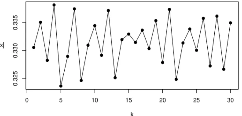
We close with a numerical example. Figure4.4shows an approximate solution of Equation (1.1) with an initial condition in M, where the parameters are as in (C) above. The delay functional is derived from the function G1/2 introduced in Remark3.3. The solutionx is the black line; the blue line shows the value of the delayd(xt).
The “irregular” behavior of the solution is not really visible at this scale. Figure4.5shows the (numerically approximated) absolute values ofx at the first several positive critical points ofx, wherexis the solution graphed in Figure4.4.
0 2 4 6 8 10
−0.3−0.10.10.3
TIME
Figure 4.4: Numerical approximation of a solutionxand the functiont 7→d(xt).
0 5 10 15 20 25 30
0.3250.3300.335
k
|x|
Figure 4.5: Numerically approximated value of |x| at the kth positive critical point ofx, 1≤ k≤30.
Acknowledgements
We thank the referee for a careful reading of the manuscript, and for helpful suggestions.
References
[1] J. Banks, J. Brooks, G. Cairns, G. Davis, P. Stacey, On Devaney’s definition of chaos,Amer. Math. Monthly99(1992), No. 4, 332–334.https://doi.org/10.2307/2324899;
MR1157223;Zbl 0758.58019
[2] R. L. Devaney,An introduction to chaotic dynamical systems, Benjamin/Cummings, Menlo Park, 1986.MR0811850;Zbl 0632.58005
[3] K. G. Grosse-Erdmann, A. P. Manguillot,Linear chaos, Universitext, Springer, London, 2001.https://doi.org/10.1007/978-1-4471-2170-1;MR2919812;Zbl 1246.47004 [4] B. B. Kennedy, A periodic solution with non-simple oscillation for an equation with
state-dependent delay and strictly monontonic negative feedback, preprint.
[5] B. Lani-Wayda, H.-O. Walther, Chaotic motion generated by delayed negative feedback, Part I: A transversality criterion, Differential Integral Equations8(1995), No. 6, 1407–1452.
MR1329849;Zbl 0827.34059
[6] B. Lani-Wayda, H.-O. Walther, Chaotic motion generated by delayed negative feedback, Part II: Construction of nonlinearities,Math. Nachr.180(1996), 141–211.https://doi.org/
10.1002/mana.3211800109;MR1397673;Zbl 0853.34065
[7] B. Lani-Wayda, H.-O. Walther, A Shilnikov phenomenon due to state-dependent delay, by means of the fixed point index,J. Dynam. Differential Equations28(2016), No. 3–4, 627–
688.https://doi.org/10.1007/s10884-014-9420-z;MR3537351;Zbl 1352.34100
[8] J. Mallet-Paret, Morse decompositions for delay differential equations, J. Differential Equations 72(1988), No. 2, 270–315. https://doi.org/10.1016/0022-0396(88)90157-X;
MR0932368;Zbl 0648.34082
[9] J. Mallet-Paret, G. R. Sell, The Poincaré–Bendixson theorem for monotone cyclic feedback systems with delay, J. Differential Equations 125(1996), No. 2, 441–489. https:
//doi.org/10.1006/jdeq.1996.0037;MR1378763;Zbl 0849.34056
[10] H. Peters, Chaotic behavior of nonlinear differential-delay equations, Nonlinear Anal. 7(1983), No. 12, 1315–1334. https://doi.org/10.1016/0362-546X(83)90003-2;
MR0726475;Zbl 0547.34064
[11] H. W. Siegberg, Chaotic behavior of a class of differential-delay equations, Ann. Mat.
Pura Appl. (4) 138(1984), 15–33. https://doi.org/10.1007/BF01762537; MR0779536;
Zbl 0568.34057
[12] H.-O. Walther, Algebraic-delay differential systems, state-dependent delay, and tempo- ral order of reactions, J. Dynam. Differential Equations 21(2009), No. 1, 195–232. https:
//doi.org/10.1007/s10884-009-9129-6;MR2482014;Zbl 1167.34026
[13] H.-O. Walther, Complicated histories close to a homoclinic loop generated by variable delay,Adv. Differential Equations19(2014), No. 9–10, 911–946.MR3229602;Zbl 1300.34162 [14] H.-O. Walther, A homoclinic loop generated by variable delay, J. Dynam. Differential
Equations27(2015), No. 3–4, 1101–1139.https://doi.org/10.1007/s10884-013-9333-2;
MR3435147;Zbl 1339.34077
[15] H.-O. Walther, Merging homoclinic solutions due to state-dependent delay,J. Differen- tial Equations259(2015), No. 2, 473–509.https://doi.org/10.1016/j.jde.2015.02.009;
MR3338308;Zbl 1326.34107