Hopf bifurcation analysis of

Hopf bifurcation analysis of

scalar implicit neutral delay differential equation

Li Zhang

and Gábor Stépán

1State Key Laboratory of Mechanics and Control of Mechanical Structures, Nanjing University of Aeronautics and Astronautics, 29 Yudao Street, Nanjing, 210012, China

2Department of Applied Mechanics, Budapest University of Technology and Economics, M ˝uegyetem rkp. 5, Budapest, H–1521, Hungary

Received 30 December 2017, appeared 26 June 2018 Communicated by Tibor Krisztin

Abstract. Hopf bifurcation analysis is conducted on a scalar implicit Neutral Delay Differential Equation (NDDE) by means of the extension of two analytical methods: 1) center manifold reduction combined with normal form theory; 2) method of multiple scales. The modifications of the classical algorithms originally developed for explicit differential equations lead to the same algebraic results, which are further confirmed by numerical simulations. It is shown that the generalizations of these regular normal form calculation methods are useful for the local nonlinear analysis of implicit NDDEs where the explicit formalism is typically not accessible and the existence and uniqueness of solutions around the equilibrium are only assumed together with the existence of a smooth local center manifold.

Keywords: neutral delay differential equation, Hopf bifurcation, center manifold re- duction, normal form, method of multiple scales, implicit differential equations.

2010 Mathematics Subject Classification: 34H20, 37L10.

1 Introduction

Neutral Delay Differential Equations (NDDE) are a class of equations whose rate of change of state depends not only on the state at present and earlier instances, but also on the rate of change of the state at earlier instances [5]. We consider the simple nonlinear scalar NDDE

˙

x(t) =ax˙(t−1) +bx(t−1) +cx˙³(t−1), (1.1) with non-zero parameters a, b, c ∈ R, where the nonlinear term cx˙³(t−1) indicates that equation (1.1) is an implicit differential equation as the highest derivative appears also with its 3rd power. What makes the problem even more intricate is the fact that the nonlinearity involves the delayed term of the first derivative. This means that however simple equation (1.1) is, it is not possible to express it in the NDDE form

d

dt(x(t)−g(x(t−1))) = f(x(t),x(t−1)), (1.2)

BCorresponding author. Email: zhangli@nuaa.edu.cn

as defined in [5] (see Section 12, Definition 1.1), which can be considered as the general explicit form of NDDEs. However, these implicit NDDEs do appear in some specific tasks, such as in a nonlinear model for human balancing subjected to saturated delayed proportional-derivative- acceleration (PDA) control [10]. There is a need to see whether normal form theories and the corresponding algorithms developed for NDDEs in [8,11] are also valid for implicit NDDEs.

We consider that the existence and uniqueness of the solutions of the implicit NDDEs around the trivial solution in question are true.

This paper carries out Hopf bifurcation analysis on the implicit NDDE (1.1) with two ana- lytical methods: 1) center manifold reduction combined with normal form theory; 2) method of multiple scales. It is shown that the two analytical methods provide the same normal form and the result is also confirmed by numerical simulation. This indicates the applicability of the extension of these regular normal from calculation methods for the local bifurcation analysis of implicit NDDEs.

The rest of the paper is organized as follows. In Section 2, linear stability is analyzed and a stability chart is presented in the parameter plane(a,b). In Section 3, Hopf bifurcation analysis is carried out with the help of normal form theory and method of multiple scales together with numerical simulations, which leads to the conclusion in Section 4.

2 Linear analysis

The stability of the trivial solutionx≡0 of (1.1) is analyzed by means of the linearized system

˙

x(t) =ax˙(t−₁) +bx(t−₁)_{. (2.1)} The corresponding characteristic equation reads

λ(1−ae^−λ)−be^−λ=0 (2.2)

for the characteristic exponentλ ∈ C. According to the D-subdivision method, substitution of λ = γ+iω into the characteristic equation (2.2) and then decomposition into real and imaginary parts yield

Re :γ+ ((−aγ−b)cosω−aωsinω)e^−γ =0 , (2.3) Im :ω+ ((aγ+b)sinω−aωcosω)e^−γ =0 . (2.4) If |a| > 1, the characteristic equation (2.2) has infinitely many characteristic exponents with positive real parts and the linear system is always unstable [6]. Therefore, only the case|a|<1 is studied here. By substituting the critical characteristic exponentλ_c =iω_c into (2.2), that is, by substitutingγ=0 into equations (2.3) and (2.4), the D-curves in the parameter plane(a,b) are obtained as

b_c =0, ifω_c=0 , (2.5)

and

ac =cosωc, bc= −ωcsinωc, ifωc >0 . (2.6) The root tendency along the D-curves is needed for determining the stability area and also the number of unstable exponents. By taking the partial derivative of (2.2) with respect to b, one gets the root tendency

α:= ^dλ(b) db

b=bc

= ¹

iωcac−ac+bc+e^iωc . (2.7)

Along the D-curveb_c =0 when ω_c =0, α= ^dλ(b)

db b=₀

= ¹

1−a_c >0 , (2.8)

which indicates that a real characteristic root crosses the imaginary axis from left to right through λ = 0 when b increases through b_c = 0, i.e. the number of unstable characteristic roots increases by 1. Along the D-curves (2.6) whenω_c 6=_0,

Reα=Re dλ(b) db

b=bc

= − ^ωcsinωc b_c²+ (a_cω_c+sinω_c)² (<0, ω_c ∈(2kπ,(2k+1)π)

>0, ω_c ∈((2k+1)π,(2k+2)π), k=0, 1, 2, . . .

(2.9)

which provides another clue for determining the number of unstable characteristic roots as Reα>0 (<0)suggests that a pair of complex characteristic roots crosses the imaginary axis from left to right (from right to left), i.e. the number of unstable characteristic roots increases (decreases) by 2.

For the linear NDDE (2.1), exponential stability only exists when

−^p1−a²arccosa< b<0 (2.10) since the number of unstable exponents is 0, as shown in Fig. 2.1. At the stability boundary b_c = −^p1−a_c²arccosa_c (the red line in Fig. 2.1), only a pair of imaginary roots ±iω_c (0 <

ω_c < π) exists while all other exponents have negative real parts and the root tendency is Reα < 0, which guarantee [4] the occurrence of Hopf bifurcation to be studied in the next section .

Figure 2.1: Stability chart of the linear NDDE (2.1) with the number of unsta- ble characteristic exponents. Grey area indicates stable region. Red line is the stability boundary where Hopf bifurcations occur in the nonlinear NDDE (1.1).

3 Hopf bifurcation analysis

Suppose that there exists a smooth local center manifold embedded in the phase space of the implicit NDDE (1.1) at the zero solution. Hopf bifurcation analysis is carried out for the implicit NDDE (1.1) by centre manifold reduction combined with normal form calculation then also by the method of multiple scales. To analyze the effect of varying b on system dynamics, the bifurcation parameterµis chosen as

b=b_c+µ. (3.1)

3.1 Centre manifold reduction combined with normal form calculation Rewrite the scalar equation (1.1) into the following operator form:

d

dtDx_t= L₀x_t+ (Lx_t−L₀x_t) +G(x˙_t), (3.2) wherex_t(θ)≡ x(t+θ), −1 ≤ θ ≤0, x_t ∈ C= C([−1, 0],R)is the Banach space of uniformly continuous functions from[−1, 0]toRwith the uniform norm,D,L₀andLare bounded linear operators fromCtoR,Dxt= xt(0)−acxt(−1),L0xt =bcx(t−1), Lxt−L0xt =µx(t−1), and the nonlinear partG(x˙_t) =cx˙³_t(−1). The solution of the linearized equation

d

dtDx_t= L₀x_t (3.3)

defines aC⁰ semigroup T(t)on C([−1, 0],R), T(t)φ= x^φ_t,t ≥ 0 . The infinitesimal generator Aassociated with T(t)is given byAφ= φ^˙ and has domain

Dom(A) =

φ∈C: dφ

dθ ∈C, Ddφ dθ = Lφ

. (3.4)

The spectrumσ(A)of Acoincides with its point spectrum if and only if it satisfies the corre- sponding characteristic equation (2.2). DefineC^∗ =C([0, 1],R). Consider the adjoint bilinear form onC^∗×C:

(_ψ,φ) = (ψ(₀)−a_cψ(₁))φ(₀) +a_c Z ₀

−1

ψ(s+₁)φ⁰(s)ds+b_c Z ₀

−1

ψ(s+₁)φ(s)ds, (3.5) which is the specific form deduced also in [9] from the general case given in [5]. Let A^∗ denote the adjoint operator of Awith respect to the bilinear form defined in Equation (3.5), i.e.,A^∗ _: C^∗ →C^∗, so that(_ψ,Aφ) = (A^∗_ψ,φ)holds for allφ∈ _Dom(A)_andψ ∈_Dom(A^∗)_. Let Λ = {iωc,−iωc}. There exist two subspaces P_Λ and Q_Λ splitting the spaceC, invariant underT(t), such thatC= P_Λ^LQ_Λ. A basis Φof P_Λ is given by

Φ(θ) = _e^iωcθ _e^−iωcθ _(3.6)

and a basisΨfor the dual spaceP_Λ^∗∗ can be expressed as Ψ(ξ) =

βe^−iωcξ βe^iωcξ

(3.7) whereβ=αe^iωc, so that(_Ψ,Φ) =I is the unit matrix, andT(t)_Φ=_Φe^Btwhere

B=

iω_c 0 0 −iω_c

. (3.8)

To write equation (3.2) as an infinite dimensional ordinary differential equation (ODE), the infinitesimal generatorAis extended to an operator ˜Aby

A˜φ= Aφ+X₀[L₀φ−Dφ⁰], φ⁰ = ^dφ

dθ (3.9)

ontoBC, the space of functions, which are uniformly continuous on[−1, 0)and with a possible finite jump discontinuity at 0, where

X0(θ) =

(0, −1≤ θ<0,

I, θ =0. (3.10)

Functionsψin BCcan be represented asψ= φ+X₀ζ, whereφ∈ C,ζ ∈R. The bilinear form (3.5) can be extended toC^∗×BCby setting (ψ,X₀) =ψ(0). LetΠ: BC→ Pbe the projection defined as Π(φ+X₀ζ) = _Φ[(_Ψ,φ) +_Ψ(₀)ζ]_{. Then} BC = P^LkerΠ and let Q ⊂ _{ker Π.}

Dom(A) =^˜ C¹([−1, 0],R), which makes sure that it is compatible with the domain of equation (3.2). The abstract ODE on the space BCis of the form:

˙

xt =A^˜xt+X₀((Lxt−L₀xt) +G(x˙t)), (3.11) Decompose xt(θ) = _Φ(θ)y(t) +zt(θ) where y(t) ∈ _R², zt ∈ Q. One obtains the following decomposition of the neutral system

˙

y= By+_Ψ(0) µ(_Φ(−1)y+z_t(−1)) +c(_Φ(−1)y˙+z˙_t(−1))³ ,

˙

z_t=A^˜z_t+ (I−_Π)X₀ µ(_Φ(−1)y+z_t(−1)) +c(_Φ(−1)y˙+z˙_t(−1))³ ,

˙ µ=0 .

(3.12)

The normal form analysis is based on a recursive sequence of nonlinear transformations.

As non-resonance condition relative to Λ is satisfied [3,8], there exists a formal nonlinear transformation

(y=y˜+V¹(y,˜ µ),

zt =z˜t+V²(y,˜ µ,) ^(3.13) such that a local manifold satisfies ˜zt = 0 and the normal form on this invariant manifold yields the following two dimensional ODE

˙˜

y= By˜+g(y, 0,˜ µ). (3.14) The third-order normal form is needed for the study of Hopf bifurcations. Based on similar deduction as in [11], the simpler form of the second-order nonlinear term g2(y, 0,˜ µ)and the third-order nonlinear term g₃(y, 0,˜ µ)can be obtained by the following recursive formula:

g_j(y, 0,˜ µ) =_Ψ(0)K_j−

j−1 k

∑

D_y˜V_k¹(y,˜ µ)g_j+1−k(y, 0,˜ µ)−(D_y˜V_j¹(y,˜ µ)By˜−BV_j¹(y,˜ µ)), (3.15) where

K2= (e^−iωcy˜₁+e^iωcy˜2)µ,

K₃= c(ie^−iωcy˜₁ω_c−ie^iωcy˜₂ω_c)³+w(y˜₁µ², ˜y₂µ²),

withw(y˜₁µ², ˜y₂µ²)representing terms related toµ²which are not expressed here in details as they are not necessary for the Hopf bifurcation analysis. The third-order normal form is then obtained as follows

y˙˜₁

˙˜

y₂

≈

iωc 0 0 −iω_c

˜ y₁

˜ y₂

+

αy˜₁µ+_∆y˜²₁y˜2

αy˜₂µ+_∆y˜₁y˜²₂

(3.16) where∆=3 iαcω_c³. Through the change of variables

y˜₁= ¹

2(ρcosϕ−iρsinϕ), ˜y2 = ¹

2(ρcosϕ+iρsinϕ), (3.17) equation (3.16) is transformed into the polar form

˙

ρ=Reα ρµ+ ¹

4Re∆ρ³, (3.18)

where Reα>0 forω_c ∈(0, π)as given in equation (2.9) and Re∆= ^3cωc

3(a_cω_c+_sinω_c)

b²_c+ (acωc+sinωc)^{2. (3.19)} If Re∆ 6= 0 and formula (2.6) of the critical parameter values are substituted, the amplitude of the bifurcated periodic motions of equation (1.1) yields

ρ=

−^4Reα Re∆µ

¹₂

=2 s

ωcsinωc

3cω_c³(ω_ccosω_c+sinω_c)(b−bc). (3.20) The sign of Re∆ determines the sense of Hopf bifurcation: if Re∆ < 0 (Re∆ > 0), it is supercritical (subcritical), i.e. the bifurcated periodic solutions are stable (unstable). The sense of Hopf bifurcations for equations (1.1) is summarized in Table3.1.

ω_c ∈ sgn Re(_∆) Sense (0, 2.03) positive subcritical (2.03, π) negative supercritical Table 3.1: Sense of Hopf bifurcations forc>0.

3.2 Method of multiple scales

To study the small amplitude oscillation, let x(t) =√

εϕ(t), µ= εµ¯, (3.21)

where ε is a nondimensional bookkeeping parameter, 0 < ε 1. ¯µ = O(1)is the detuning parameter. Then equation (1.1) is transformed into the form

˙

ϕ(t)−acϕ˙(t−1)−bcϕ(t−1) =ε(µϕ¯ (t−1) +cϕ˙³(t−1)). (3.22) The multiple time scales are defined asT_k =ε^kt, k=0, 1, 2, . . . To study the Hopf bifurcation, a two scale expansion of the solution is assumed as

ϕ(t) = ϕ₀(T₀,T₁) +εϕ₁(T₀,T₁) +_O(ε²)_{. (3.23)}

By using the differential operators [7]

d dt = ^∂

∂T₀ +ε ∂

∂T₁ +O(ε²) =: D₀+εD₁+O(ε²), d²

dt² =: D₀²+2εD₀D₁+O(ε²),

(3.24)

the delayed terms can be expressed as

ϕ(t−1) =ϕ₀(T₀−1,T₁−ε) +εϕ₁(T₀−1,T₁−ε) +· · ·

= ϕ₀(T₀−1,T₁) +ε(ϕ₁(T₀−1,T₁)−D₁ϕ₀(T₀−1,T₁)) +O(ε²). (3.25) Substituting equations (3.23), (3.24) and (3.25) into equation (3.22) and equating the same powers ofε, a set of linear partial differential equations can be obtained in the form

D₀ϕ₀−a_cD₀ϕ_0τ−b_cϕ_0τ =0 , (3.26) D0ϕ₁−acD0ϕ_1τ−bcϕ_1τ = (_ac−bc)_D1ϕ_0τ−acD0D1ϕ_0τ+µϕ¯ _0τ−D1ϕ₀+_c(_D0ϕ_0τ)³_{, (3.27)} where ϕ_i = ϕ_i(T0,T₁),ϕ_iτ = ϕ_i(T0−1,T₁). At the stability boundary (the red line in Fig.2.1), only one pair of pure imaginary characteristic roots ±iω_c exists, while all other eigenvalues have negative real parts. All the solution terms related to eigenvalues with negative real parts decay with time. Thus, to study the long-time behavior of the system, the solution of equation (3.26) can be assumed as

ϕ₀= R(T₁)e^iωcT0 +R(T₁)e^−iωcT0. (3.28) Substituting equation (3.28) into equation (3.27), the secular term can be found

(a_c−b_c−iaω_c−e^iωc)R^˙(T₁) +3icω²_cR²(T₁)R(T₁) +µR¯ (T₁) =0 . (3.29) R˙(T₁)is determined by

R˙(T₁) = ^R(T₁)µ¯ +3icω³_cR²(T₁)R(T₁)

ia_cω_c+e^iωc−a_c+b_c . (3.30) With

y˜₁ = √¹

εR(εt)e^iωct, (3.31)

the normal form equation (3.30) is transformed to the exact same formula as the normal form equation (3.16) derived by using the centre manifold reduction and normal form theory.

3.3 Case studyac =1/√

2, c =0.1

To see whether the analytical results agree with numerical results, numerical analysis is also presented for the case a_c =1/√

2,c=0.1 with the help of collocation method combined with path-following techniques [1,2]. Based on equation (2.6), one can have

b_c =− ^π 4√

2, ω_c = ^π 4 .

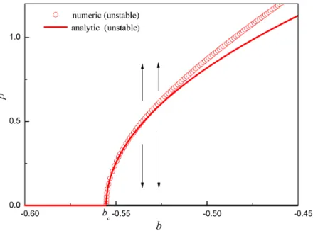
According to Table 3.1, the analysis indicates that a subcritical Hopf bifurcation occurs since ω_c ∈ (0, 2.03), which is in good agreement with the numerical result shown in Figure 3.1.

This illustrates the validity of the two normal form calculation methods for implicit NDDEs.

Moreover, two time domain simulations withb=−0.5 and different initial conditions (x₀(t)≡ 0.1;x₀(t)≡1, t∈ [−1, 0]) are presented in Figure3.2to demonstrate the characteristic of the subcritical Hopf bifurcation.

Figure 3.1: Bifurcation diagram with respect tob. a = 1/√

2. Continuous lines refer to analytical results, series of circles refer to numerical results obtained by collocation method and path following. Red color represents unstable branches.

Figure 3.2: Time history with different initial conditions;x₀(t)≡0.1 (black line), x₀(t)≡1 (red line),t∈[−1, 0],a =1/√

2,b= −0.5.

4 Conclusion

It is shown that both center manifold reduction combined with normal form theory and the method of multiple scales can be extended and applied for Hopf bifurcation analysis of im- plicit NDDEs.

Acknowledgements

The work of LZ was supported by the National Natural Science Foundation of China under Grants No. 11302098 and No. 11772151, the work of GS was also supported by the Research Fund of the State Key Laboratory of Mechanics and Control of Mechanical Structures (NUAA) under Grant No. MCMS-0116K01. LZ gratefully acknowledges financial support from China Scholarship Council.

References

[1] D. A. W. Barton, B. Krauskopf, R. E. Wilson, Collocation schemes for periodic solutions of neutral delay differential equations, J. Differ. Equ. Appl. 12(2006), No. 11, 1087–1101.

https://doi.org/10.1080/10236190601045663;MR2271819

[2] K. Engelborghs, T. Luzyanina, G. Samaey,DDE-BIFTOOL v. 2.00: A Matlab package for bifurcation analysis of delay differential equations, 2001.

[3] T. Faria, L. T. Magalhães, Normal forms for retarded functional-differential equations with parameters and applications to Hopf bifurcation,J. Differential Equations122(1995), No. 2, 181–200.https://doi.org/10.1006/jdeq.1995.1144;MR1355888

[4] J. Guckenheimer, P. Holmes, Nonlinear oscillations, dynamical systems and bifurca- tions of vector fields, Springer-Verlag, New York, 1983. https://doi.org/10.1007/

978-1-4612-1140-2;MR1139515

[5] J. K. Hale, Theory of functional differential equations, Applied Mathematical Sciences, Vol. 3, Springer-Verlag, New York, 1977.https://doi.org/10.1007/978-1-4612-9892-2;

MR0508721

[6] W. Michiels, S. Niculescu, Stability and stabilization of time-delay systems: an eigenvalue- based approach, SIAM, Philadelphia, 2007. https://doi.org/10.1137/1.9780898718645;

MR2384531

[7] A. H. Nayfeh, D. T. Mook,Nonlinear oscillations, Wiley, New York, 1979.MR549322 [8] M. Weedermann, Normal forms for neutral functional differential equations, in: Topics in

functional differential and difference equations (Lisbon, 1999), Fields Inst. Commun., Vol. 29, 2001, pp. 361–368.MR1821791

[9] M. Weedermann, Hopf bifurcation calculations for scalar neutral delay differential equa- tions,Nonlinearity 19(2006), 2091–2102. https://doi.org/10.1088/0951-7715/19/9/005 MR2256652

[10] L. Zhang, G. Stépán, T, Insperger, Saturation limits the contribution of acceleration feedback to balancing against reaction delay,J. R. Soc. Interface15(2018), No. 138.https:

//doi.org/10.1098/rsif.2017.0771

[11] L. Zhang, H. L. Wang, H. Y. Hu, Symbolic computation of normal form for Hopf bifur- cation in a neutral delay differential equation and an application to a controlled crane, Nonlinear Dyn. 70(2012), No. 1, 463–473. https://doi.org/10.1006/jmaa.1993.1212;

MR2991286