Magnetic Methods of Analysis
B Y
A. R. K A U F M A N N
Department of Metallurgy, Massachusetts Institute of Technology, Cambridge, Μ assachusetts
CONTENTS
Page
1. Introduction 230 2. Definitions and Units 230
2.1. Magnetic Field 230 2.2. Intensity of Magnetization and Susceptibility 231
2.3. Flux 231 2.4. Permeability 232 3. Magnetic Energy and Force 232 4. Magnetic Materials 233
4.1. Diamagnetism 233 4.2. Paramagnetism 233 4.3. Ferromagnetism 233 5. Demagnetizing Field 236 6. Production of Magnetic Fields 237
6.1. Electromagnets 237 6.2. Solenoids 237 6.3. Permanent Magnets 238
6.4. Earths Field 239 7. Measurement of Magnetic Fields 239
7.1. Search Coil 239 7.2. Flux Meter 240 7.3. Standard Substances 240
7.4. Bismuth Wire 240 7.5. Current Methods 241 8. Apparatus for Magnetic Measurements 241
8.1. Force Measurements 241 8.1.1. Curie Method 241 8.1.2. Gouy Method 242 8.1.3. Quincke Method 242 8.1.4. General Precautions 243 8.2. Magnetometer Methods 244
8.2.1. Pendulum 244 8.2.2. Compass 244 8.3. Torque Methods 245 8.4. Induction Methods 245 8.5. Alternating Current Methods 246
229
230 A. R . K A U F M A NN
9. Applications of Magnetic Analysis 9.1. Oxygen in Air
9.2. Carbon in Steel
9.3. Phase Transformations... . 9.4. Geological Applications... . 9.5. Single Crystals
9.6. Molecular Structure 9.7. Magnetic Titrations References
Page 247 247 248 248 249 250 250 252 253 1. IN T R O D U C T I ON
T h e magnetic properties of m a t t e r h a v e been studied for m a n y years by numerous investigators. A large n u m b e r of research methods a d a p t e d to this work have been developed, with almost every worker incorporating variations of design in his own a p p a r a t u s . This situation exists because t h e large range of phenomena a n d experiments covered b y magnetic studies have precluded t h e construction of a s t a n d a r d piece of test equipment. T h e following article will cover t h e broad field of magnetic test methods insofar as t h e y m a y be of use t o t h e analyst, without mentioning certain techniques used either in t h e realm of pure physics or in connection with t h e detailed applications of ferromagnetic materials in commercial equipment.
Magnetized bodies will exert forces on each other which m a y be described in terms of magnetic poles located on t h e surface of t h e bodies.
There are two types of poles, n o r t h and south; like poles repel each other and unlike poles a t t r a c t . A n o r t h pole is one t h a t would move in a northerly direction in the e a r t h ' s field. T h e force, F, between two poles of strength pi a n d p2, separated by a distance, r, acts along a line drawn between t h e m a n d is given b y t h e equation F = where μ is t h e permeability (to be discussed below) of t h e medium surrounding t h e poles. Two poles of unit strength will exert a force of 1 dyne on each other when μ = 1 (as in a vacuum) and r = 1 cm.
A magnetized body produces a magnetic field, H, whose strength at any point is given b y t h e force it exerts on a unit pole placed in a v a c u u m at t h a t point (the unit is t h e oersted). T h e direction of t h e field is t h a t in which it causes a north pole to move. A unit field exerts a force of 1 dyne on a unit pole. I t follows from this t h a t a unit pole produces a unit field at a distance of 1 cm.
2. DE F I N I T I O NS A N D UN I TS
2.1. Magnetic Field
MAGNETIC METHODS OF ANALYSIS 231 2.2. Intensity of Magnetization and Susceptibility
Two magnetic poles of equal strength a n d of opposite kind, when separated b y a distance Z, form a magnetic m o m e n t (dipole) of strength m = pi. T h e intensity of magnetization, J, of a body is defined as its magnetic m o m e n t per cubic centimeter. W h e n 7 is produced through the action of a magnetic field, t h e volume susceptibility, K, of t h e material is defined as I/H = K. T h e magnetic m o m e n t per gram, σ, a n d t h e mass susceptibility, χ, are obtained by dividing 7 or Κ b y t h e density, respectively. T h e corresponding quantities for a gram molec
ular weight of material are obtained by multiplying σ or χ b y t h e gram molecular weight.
2.8. Flux
A magnetic field m a y be represented b y drawing lines t h r o u g h space indicating t h e direction in which a unit pole would move at a n y point a n d with t h e strength of t h e field being indicated b y t h e density of lines (the unit is t h e gauss). A unit field corresponds (by convention) t o a density of one line per square centimeter of area perpendicular t o t h e line. F r o m this it follows t h a t 4π lines originate from each unit pole since such a pole produces unit field strength over t h e surface of a sphere of 1 cm. radius. A cube of material 1 cm. on a side, magnetized t o an intensity 7, has a magnetic m o m e n t equivalent t o t h a t of t h e same cube with magnetic poles of strength ρ = 7 located on t w o opposite faces.
I n other words, 7 has t h e dimensions of magnetic m o m e n t per cubic centimeter or pole strength per square centimeter.
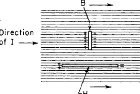
If a disclike cavity (see Fig. 1) is created inside a body uniformly magnetized t o a n intensity 7, with t h e plane of t h e disc normal t o t h e direction of 7, n o r t h poles of strength 7 per centimeter squared will be formed on one face of t h e cavity with south poles of t h e same strength on t h e other face. Thus, these poles will produce a field of strength 4π7 across t h e cavity t h a t is due t o t h e magnetization of t h e material. I n addition there will be a field due t o t h e magnetizing field, i7, which exists within t h e body a t t h a t point. This field is not necessarily t h e same in strength as t h e field t h a t would exist at t h a t point if t h e specimen were removed since there m a y be a demagnetizing field (see discussion below).
T h e t r u e value of Η a t a point within a body could be determined b y measuring t h e field in t h e middle of a long, needlelike cavity, as shown in Fig. 1.
T h e sum Η + 4π7 = jB is k n o w n as t h e magnetic flux in a body. I t is a p p a r e n t t h a t B, 77, a n d 7 h a v e t h e same dimensions, b u t in spite of this the units of t h e first two are gauss a n d oersted, respectively, while 7
232 A. R . K A U F M A NN
has no commonly used unit. I t is customary for engineers t o use t h e q u a n t i t y Β since this measures t h e useful flux produced in magnetic equipment, while scientists prefer t h e q u a n t i t y I or σ, since these refer directly t o a property of t h e material.
Β
D i r e c t i o n of I >
FIG. 1. Β and Η inside an inductively magnetized specimen.
2.4. Permeability
T h e ratio Β/Η — μ = 1 + 4 π Κ is known as t h e permeability. This q u a n t i t y is used b y engineers in preference t o Κ for t h e same reasons t h a t t h e y prefer Β t o / . I t is a p p a r e n t t h a t b o t h μ a n d K, as defined in this article have no dimensions. T h e μ defined here is assumed t o be t h e same as in t h e introductory p a r a g r a p h of section 2 b u t a p p a r e n t l y there is no w a y of proving this experimentally (2).
3. MA G N E T IC EN E R GY A N D FO R CE
T h e m u t u a l energy of a dipole a n d t h e field producing a p p a r a t u s is determined b y t h e orientation of t h e dipole with respect t o t h e field, t h a t is, Ε = — mH cos 0 where 0 is t h e angle between t h e axis of t h e dipole a n d t h e field direction. This follows from t h e fact t h a t t h e work required to bring t h e n o r t h pole of t h e dipole into t h e field is equal a n d opposite to t h a t required t o bring t h e south pole into t h e field, except for t h e small difference determined b y t h e orientation with respect t o t h e field. T h e m u t u a l energy of a magnetized body a n d t h e field a p p a r a t u s is — IHV cos 0, where V is t h e volume in cubic centimeters. T h e t o r q u e acting
dE
T h e force on t h e body in t h e a>direc- on t h e body is = IHV sin 0.
tion is dE
dx V. If t h e specimen is
(
Hx dH^j. F o r nonisotropic specimens t h e energy a n d
+ H y -τ— " Γ Hz
dx
dHz dx
force relationships are more complicated (3).
M A G N E T IC M E T H O DS O F A N A L Y S IS 233 W h e n magnetization is induced by a field, t h e internal energy change of t h e specimen is V IdH (6), which is t h e area between t h e m a g netization curve a n d t h e J-axis. F r o m this result, it is easy t o show.that for cyclic magnetization t h e area within t h e hysteresis loop equals t h e loss of energy per cycle.
There are t h r e e t y p e s of magnetic behavior: diamagnetic, p a r a m a g netic a n d ferromagnetic. N o a t t e m p t will be m a d e t o give a discussion of these phenomena from an atomic standpoint since t h e subject is very extensive a n d is covered in s t a n d a r d works on magnetism. A brief reference t o t h e atomic theory is given in Section 9.6.
For a diamagnetic material, Κ is negative a n d hence t h e magnetiza
tion is antiparallel t o t h e applied field, H. T h e value of Κ will be of t h e order of 10~6 as shown b y a few examples listed in Table I. Κ is strictly independent of Η a n d varies only slightly with t h e t e m p e r a t u r e (40). Appreciable t e m p e r a t u r e dependence of Κ for diamagnetic materials indicates t h a t there is a paramagnetic component of t h e magnetization which is not great enough, however, t o m a k e t h e resultant magnetization paramagnetic.
A paramagnetic material has a positive Κ of t h e m a g n i t u d e 10~6 to 10~4 a t room t e m p e r a t u r e (Table I) a n d likewise is independent of Η at room t e m p e r a t u r e . T h e magnetization will be parallel t o H. M a n y paramagnetic susceptibilities, particularly of nonmetals, v a r y roughly as t h e reciprocal of t h e absolute t e m p e r a t u r e a n d hence m a y become very large at low t e m p e r a t u r e s . A t such t e m p e r a t u r e s Κ m a y become dependent on H, b u t t h e magnetization will always be reversible.
Ferromagnetism is a special case of paramagnetism in t h e sense t h a t Κ is positive (for virgin magnetization) a n d I is parallel t o Η when Η is large. However, Κ will v a r y tremendously with Η a n d can have large values as shown in Table I. This m e a n s t h a t I can have large values at relatively small values of H. T h e magnetization, J, at low field strengths can be at any angle t o Η depending on numerous factors such as shape and orientation of t h e specimen, structure a n d orientation of t h e crystals comprising t h e specimen, a n d previous magnetic history. M o s t ferro-
4. MA G N E T IC MA T E R I A LS
4.1. Diamagnetism
4.2. Paramagnetism
4.8. Ferromagnetism
234 A. R. KAUFMANN
magnetic materials can retain some magnetization in zero field and this distinguishes t h e m fundamentally from paramagnetic substances.
T h e magnetization of a ferromagnetic will substantially reach a limiting value, known as t h e saturation value, I8, in fields of several thousand oersted. I t is found t h a t I8 decreases with increasing tempera- ture and goes rather a b r u p t l y to almost zero at a critical t e m p e r a t u r e , Tc, known as t h e Curie t e m p e r a t u r e . At still higher t e m p e r a t u r e s t h e magnetization is essentially paramagnetic in n a t u r e .
Typical magnetization curves for t h e three types of magnetic behavior are shown schematically in Fig. 2. T h e virgin curve for t h e ferro-
+1
^ F e r r o m a g n e t ic
^ - P a r a m a g n e t ic
/ ?
/ ^ D i a m a g n e t i c
- I
FIG. 2. Magnetization curves for diamagnetic, paramagnetic and ferromagnetic materials.
magnetic case is seen t o be greatly different from t h e curve obtained on succeeding reversals of t h e field. This phenomenon is known as hysteresis and is of great consequence b o t h in practical applications a n d to the analyst. I t is obvious t h a t previous magnetic history would need to be considered in making analytical deductions from measurements on a ferromagnetic material.
After a ferromagnetic material reaches its saturation value, there will be a further almost linear increase in magnetization with field. This effect is small at t e m p e r a t u r e s considerably below t h e Curie t e m p e r a t u r e b u t m a y be quite appreciable in t h e neighborhood of Tc. T h e t r u e value of I8 can be found b y extrapolating t h e linear behavior in very high fields (above 20,000 oersted) back to t h e zero field axis a n d obtaining t h e intercept as shown in Fig. 2. At a given t e m p e r a t u r e I8 is a character- istic of t h e material a n d could be used as an aid in identification.
MAGNETIC METHODS OF ANALYSIS 235 TABLE I
Volume Susceptibility of Various Substances Substance Tempera
ture °C. Κ X 106 Remarks
Sodium chloride Copper
Water Ethyl alcohol Air
Oxygen Aluminum Manganese Ferric chloride Iron
20 20 18 20 20 20 18 20 20
5 Χ 108 to 101 0
- 1 . 0 8 - . 7 6 - . 7 2 0 - . 5 8 + .029 + .143 + 1.75 + 7 3 + 2 4 0
Ferromagnetic 760 mm.
760 mm.
T h e magnetization curve and hysteresis loop of a ferromagnetic m a t e rial are of such great technical importance t h a t m a n y features of t h e curves have received specific names and symbols as shown in Fig. 3, where Β = Η + 47Γ/ is plotted against H. T h e slope of a line drawn from t h e
origin to a n y point on t h e virgin curve gives t h e permeability at t h a t point. T h e slope of t h e curve a t t h e origin is known as t h e initial per
meability, while t h e slope of t h e virgin curve at a n y other point is known as t h e differential permeability. If, at a n y value of Η a small variation of field, AH, is carried out m a n y times, t h e q u a n t i t y AB/AH, k n o w n as the reversible permeability, m a y be obtained and this will be greatly different from t h e differential permeability. T h e intercept of t h e demag
netization curve with t h e #-axis is known as t h e remanence, Br, while t h e
.J
Η
FIG. 3. Illustration of remanence, Br, and coercive force Hc.
236 A. R . K A U F M A NN
intercept on the //-axis is t h e coercive force, Hc. T h e remanence a n d coercive force have definite values only if t h e magnetization is carried t o saturation.
5. DE M A G N E T I Z I NG FI E LD
A magnetized body will have free poles on its surface a t t h e places where t h e flux either enters or leaves t h e body. These poles will create a magnetic field, as discussed above, which will extend in all directions through space. Within t h e body itself this field, k n o w n as t h e demag
netizing field, will act in a direction more or less opposite t o t h a t of t h e magnetization a n d t o t h e field producing t h e magnetization. I n a specimen of irregular shape t h e direction a n d m a g n i t u d e of t h e demag
netizing field, H', will obviously be h a r d t o specify. I n t h e case of a n oblate or prolate spheroid, however, which is uniformly magnetized parallel t o one of t h e axes, it can b e shown t h a t H' n o t only is uniform throughout t h e body b u t also is proportional t o / a n d is antiparallel t o it. Thus, the t r u e field inside such a b o d y is Η — Η' = Η — DI.
T h e constant D can be computed from equations given in books on magnetism (36). T h e value of D is £π for a sphere a n d 4π for magnetiza
tion perpendicular to t h e plane of a thin disc, showing t h a t t h e demag
netizing field can be very i m p o r t a n t when J is large as in a ferromagnetic material. The coefficient of demagnetization along t h e axis of long t h i n ellipsoids becomes small as the ratio of length t o diameter is increased, as shown in t h e second column of Table I I . T h e q u a n t i t y , m, in this table is t h e ratio of length t o diameter for t h e ellipsoids or cylinders.
Measurements are often m a d e on specimens in t h e form of cylinders and for this case empirical values of D , which presumably apply only t o t h e middle region of t h e rod, h a v e been determined a n d are given in t h e third column of Table I I (31).
TABLE II Demagnetization Factors
m D D
m Ellipsoid Cylinder
1 4.188 δ .701 10 .255
20 .085 .067
30 .043 .034
50 .018 .014
100 .0054 .0045 500 .0003 .00018
M A G N E T I C M E T H O D S O F A N A L Y S I S 237
6 . P R O D U C T I O N O F M A G N E T I C F I E L D S
6.1. Electromagnets
Electromagnets are familiar t o most people a n d h a v e been discussed in m a n y places (4). A m a x i m u m of a b o u t 21,000 oersted m a y be obtained using a n iron core a n d flat pole pieces, while with tapered poles a n d special steels a b o u t 35,000 oersted from t h e iron alone m a y be obtained.
B y placing t h e magnetizing coils in line with a n d close t o t h e pole pieces a further increase in field is possible depending on how m u c h current is used. I n this w a y a b o u t 45,000 oersted m a y be obtained with a m o d e r a t e size of installation, while 70,000 oersted has been reached in extreme cases.
T h e distribution of field between t h e pole pieces m a y be quite com
plex a n d ordinarily will be uniform only over a small region. Special shapes of pole pieces can be used t o obtain specific field distributions, b u t t h e shaping is difficult t o determine except b y trial a n d error. Cir
cular poles with slightly concave faces have been used t o give uniform fields a n d poles of unequal size t o produce uniform field gradients (9).
W h e n placing a strongly magnetic specimen in t h e gap of a m a g n e t it is i m p o r t a n t t o remember t h a t t h e specimen m a y react on t h e m a g n e t a n d alter t h e strength a n d distribution of t h e field.
6.2. Solenoids
T h e magnetic field produced b y a known distribution of electric currents can be accurately calculated in most cases (24). B y this m e a n s s t a n d a r d fields for t h e calibration of magnetic equipment can be produced a n d also fields with accurately k n o w n uniformity or gradients. A very long helix of wire with η t u r n s per centimeter, which carries a current of i amperes will produce a uniform field a t its center of strength of Η = Απητ. Formulas giving t h e strength a n d distribution of field for shorter coils m a y be found in m a n y references (13).
A uniformly wound multiple-layer solenoid is very convenient for pro
ducing fields u p t o a b o u t 500 oersted. For greater field strengths in continuous service it becomes necessary t o provide cooling. T h r o u g h t h e use of enough power a n d enough ingenuity in removing heat, it is possible t o produce continuous fields u p t o 100,000 oersted (5) or fields u p t o 300,000 for a fraction of a second (37).
Fields of great uniformity over a large space m a y be produced through t h e use of Helmholtz coils. These consist of two circular coils spaced a n d dimensioned as shown in Fig. 4 with equal currents flowing in t h e same sense in t h e two coils. T h e field so produced is given closely b y
238 A. R. KAUFMANN
the equation Η = ^ — where ι is the current in amperes, Ν is the number of t u r n s in each coil, a n d R is t h e radius of t h e coil in centimeters.
This is an inefficient way of producing a field and, hence, t h e coils are used mostly to produce relatively weak fields such as are needed to balance out the earth's field. According t o M c K e e h a n a uniform
a_2 = 3 6 b2 31
cr
m
i i
FIG. 4. Helmholtz coils for producing uniform field.
gradient, dH/dx (23) m a y be produced by spacing t h e coils a distance Λ/3 R apart and running the currents in opposite directions.
6.3. Permanent Magnets
P e r m a n e n t magnets have found only a limited use as a field source for magnetic testing owing to t h e inability t o v a r y t h e field (except with a winding) a n d to t h e expense of t h e material required for a sizable magnet. In general, the maximum attainable field would be of t h e order of 5000 to 10,000 oersted, depending on t h e magnet material and the size of the gap. A properly designed a n d stabilized p e r m a n e n t magnet should give a much more constant field t h a n is obtainable when electric currents are required to produce the field (due to fluctuations in current) and this feature m a y be highly desirable in special cases.
M A G N E T I C M E T H O D S O F A N A L Y S I S 239 64. Earth's Field
T h e magnetic field of t h e e a r t h is uniform over large regions (unless distorted b y local magnetized material) a n d is quite constant from day t o day. For this reason it is sometimes used as a reference field, par
ticularly in t h e magnetometer a p p a r a t u s t o be described below. T h e strength of t h e horizontal component of t h e earth's field in t h e north
eastern United S t a t e s is about 0.2 oersted, while t h e vertical component is a b o u t 0.5. Observations which are m a d e in fields of this order of magnitude would obviously need t o be corrected for t h e effect of t h e e a r t h ' s field.
7.1. Search Coil
A search coil coupled t o a ballistic galvanometer t h r o u g h t h e second
ary of a m u t u a l inductance, as shown in Fig. 5, is probably t h e most
FIG. 5. Wiring diagram for search coil and ballistic galvanometer circuit.
widely used m e a n s of measuring H. If t h e component of Η perpendicular t o t h e plane of t h e coil is varied rapidly, a voltage is induced in t h e coil a n d this causes a current i\ t o flow t h r o u g h t h e galvanometer. If all of t h e current flows before t h e galvanometer has moved appreciably, t h e amplitude of swing of t h e galvanometer coil will be strictly propor
tional to t h e angular impulse imparted by t h e current t o t h e galvanometer άφ coil. T h e instantaneous voltage at t h e search coil is Ε = 10~8
dH
= 10~SNA where φ is t h e flux t h r o u g h t h e coil, Ν equals t h e n u m b e r of t u r n s in t h e search coil a n d A is t h e cross-sectional area of t h e coil in square centimeters. T h e angular impulse is proportional t o j idt
7. M E A S U R E M E N T O F M A G N E T I C F I E L D S
*— G o l v a n o m e t er
240 A. R. KAUFMANN
•8 NAAH
Ζ = c0i where Ζ is t h e total impedance of the circuit, AH is t h e change of field, θ is t h e deflection of t h e galvanometer, and c is a constant. T h e m u t u a l inductance is used t o calibrate t h e galvanometer b y breaking a current i' in t h e primary. This will cause a galvanometer deflection 02 where cd2 = ~~ ζ' · Hence, AH = ^ ^ y ^ ^*
where Μ is in henries a n d if is in amperes.
T h e flux through t h e search coil m a y be varied b y reducing Η t o zero, by pulling t h e coil from t h e field, or b y rotating t h e coil till its plane is parallel to t h e field. If t h e area of a coil is difficult t o fix, it m a y be determined b y making t h e above measurements in an accurately k n o w n field. There are m a n y details on t h e operation of a ballistic galvanometer which m a y be found in text books on. electrical measurements (34).
A galvanometer t h a t has practically no restoring force or t h a t is heavily overdamped can be used t o measure flux changes t h r o u g h a search coil without t h e necessity of making all of t h e flux change before the instrument moves (25). Such instruments in portable form can be bought commercially a n d are quite convenient for rough work. T h e y are not suitable for precise work, however, since it is difficult t o obtain accurate readings owing t o t h e small scale a n d t h e slow drift of t h e pointer.
T h e field in a p p a r a t u s used for measuring t h e susceptibility of p a r a magnetic or diamagnetic materials m a y be calibrated b y using s u b stances of known susceptibility. P u r e water with Κ = —0.720 X 10~6 at 16°C. has been used for this purpose. T h e susceptibility of para
magnetic salts varies rapidly with t e m p e r a t u r e , hence t h e t e m p e r a t u r e must be fixed when making a calibration with such materials. Some of these methods, as will be described later, give Η directly a n d others give Η -^j— a t a point. T h e technique is useful mostly for determining large fields.
T h e electrical resistance of a b i s m u t h wire varies roughly as t h e square of t h e magnetic field in which it is placed, with a 4 0 % increase being observed a t 10,000 oersted. Such wires can be m a d e quite small a n d hence are useful for field determination in a small region. I t is neces-
7.2. Flux Meter
7.3. Standard Substances
dH
7.4. Bismuth Wire
M A G N E T I C M E T H O D S O P A N A L Y S I S 2 4 1
sary t o m a i n t a i n a constant t e m p e r a t u r e since the effect varies with t e m p e r a t u r e .
7.5. Current Methods
A field can be measured b y determining t h e force which it exerts on a k n o w n electric current. T h e force, F, in dynes on a n element, ds,
Hids
of current is F = —jq- sin Θ, where θ is t h e angle between ds a n d H, a n d i is t h e current in amperes. T h e force will be a t right angles t o t h e plane defined b y t h e directions of ds a n d of H. T h e C o t t o n balance ( 3 8 ) has been used in several investigations. Another very simple arrangement consists of a uniformly wound single layer solenoid sus
pended from t h e a r m of a balance ( 1 9 ) . I n each case t h e difference of t h e field a t t h e t w o ends of t h e current carrying structure is determined.
These m e t h o d s can be used where absolute accuracy is required.
8 . A P P A R A T U S F O R M A G N E T I C M E A S U R E M E N T S
8.1. Force Measurements
8.1.1. Curie Method. T h e magnetization of a b o d y can be determined by measuring t h e translation force exerted on t h e specimen b y a n inhomo- geneous magnetic field of k n o w n strength a n d gradient. This m e t h o d is particularly a d a p t e d t o observations on diamagnetic a n d p a r a m a g netic substances since t h e induction m e t h o d s used on ferromagnetic materials are not sufficiently sensitive for this purpose. Let t h e x-axis coincide with t h e direction in which t h e force is t o be m e a s u r e d : F o r a magnetically isotropic substance t h e force on a small volume, dV, is fx = K ^Hx + Hy + Hz ^ f j dV. If t h e specimen is sus
pended from a balance along t h e axis of a solenoid, as shown in Fig. 6, /
KHX dV dH
= KVHX^£ = xwHx (w = weight of specimen), if Hz~^j~ is uniform over t h e specimen. If t h e specimen is suspended near t h e gap of
dH an electromagnet, as shown in Fig. 7, t h e force is F = xwHv - ^ p If t h e specimen is surrounded b y a gaseous or liquid medium of suscepti-
dH bility Ko, t h e force will be Fx = (K - K0)VHX ~
This procedure, k n o w n as t h e Curie method, h a s t h e a d v a n t a g e t h a t only a small sample is required a n d t h a t t h e specimen can be of irregular
dH
shape. T h e disadvantage is t h a t Η cannot be determined very
242 A. R. KAUFMANN
accurately at a point and, hence, t h e precision is usually not better t h a n a few per cent. T h e m e t h o d is capable of great sensitivity if t h e speci- men is held on a horizontal a r m which is suspended from a torsion fiber.
8.1.2. Gouy Method. If t h e specimen consists of a long cylinder of uniform cross section, A (sq. cm.), t h e force exerted on it b y a field (Fig. 8) can be found b y integration of t h e above expression over t h e
S p e c i m en
S p e c i m en
7~* —A
^ B a l a n ce
FIG. 6. Curie method for measuring suscepti- bility using a solenoid.
FIG. 7. Curie method for determining susceptibility using an electromagnet.
length of t h e specimen. T h e result is Fx = (K - K0)A
Ho
2).
T h e a d v a n t a g e of t h e G o u y m e t h o d is t h a t it is not necessary t o know dH
-jj-> and, if Hq is small compared with Hi, t h e n H0 usually can be neg-
lected. T h e disadvantage is t h a t a large specimen of uniform cross
S p e c i m en
Hf
FIG. 8. Gouy method for determining susceptibility using an electromagnet.
section is required. A long specimen is particularly disadvantageous when t h e specimen is to be either heated or cooled.
8.1.8. Quincke Method. Susceptibility measurements on liquids can be m a d e b y t h e Curie or Gouy methods but, in either case, a correction would need to be m a d e for t h e sample container. This is avoided in t h e Quincke m e t h o d where t h e liquid is contained in a stationary U t u b e with
MAGNETIC METHODS OF ANALYSIS 243 one a r m of t h e U in t h e magnetic field a n d t h e other in zero field as shown in Fig. 9. T h e level of t h e liquid will move when t h e field is t u r n e d on a n d a n observation of this change, h, or of t h e motion of a reservoir which will restore t h e original liquid level is a measure of t h e susceptibility.
T h e mass susceptibility is given b y χ = - j p + when t h e outer a r m of t h e U h a s a large enough reservoir so t h a t its level does n o t change appreciably a n d when t h e density, po, of t h e medium above t h e sample can b e neglected. I n this expression, G is t h e gravitational constant, ρ is t h e density of t h e sample, a n d χ0 is t h e susceptibility of t h e upper medium. This m e t h o d h a s t h e advantages of t h e G o u y system with t h e further feature t h a t t h e cross-sectional area need n o t b e known.
FIG. 9. Q u i n c k e m e t h o d f o r m e a s u r i n g t h e s u s c e p t i b i l i t y o f l i q u i d s .
8. I 4 . General Precautions. T h e presence of ferromagnetic impurities in a sample can produce serious error in susceptibility measurements.
T o avoid this it is necessary t o measure Κ a t a series of field strengths above about 7000 oersted a n d t h e n t o plot Κ against 1/H t o get t h e extrapolated value a t infinite field. If Γ is t h e saturation value of t h e
Γ 2Γ impurities, t h e n KH = jj + for t h e Curie method, a n d KH = ~jj
+ for t h e G o u y method.
W h e n using t h e Curie method, it is necessary t o m a k e corrections for t h e force exerted b y t h e field on t h e specimen holder a n d suspension thread. This can best be done b y correcting t h e observed force a t each field strength r a t h e r t h a n calculating a susceptibility for t h e holder.
W i t h t h e Curie or G o u y methods where t h e specimen is freely sus
pended in t h e field, t h e forces perpendicular t o t h e direction of measure
ment m a y be great enough, when Κ is large, t o deflect t h e specimen against t h e sides of t h e a p p a r a t u s . T h e only cure for this is t o use weaker fields or more homogeneous fields. When Κ is very large (as a t low temperatures), t h e equilibrium in t h e direction of measurement m a y become unstable. T h e remedy for this is t o decrease t h e sensitivity of t h e balance or t o use weaker fields.
244 A. R. KAUFMANN
There are m a n y variations of t h e methods given above, particularly with regard t o t h e means of measuring t h e force. T h e reader is referred t o s t a n d a r d works on magnetism for a more extensive discussion (39).
8.2. Magnetometer Methods
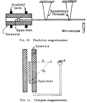
8.2.1. Pendulum. T h e magnetization of strongly paramagnetic or ferromagnetic materials can be determined b y measuring t h e transla- tional force on specimens attached to a horizontal rod suspended from
FIG. 10. Pendulum magnetometer.
^ - S o l e n o i d
FIG. 11. Compass magnetometer.
four threads as shown in Fig. 10 (14, 23). T h e specimen can be quite small b u t must be shaped into an ellipsoid in order t o h a v e a known demagnetizing factor. T h e field gradient need only be small and, hence, can be supplied with modified Helmoltz coils. If t h e .weight a n d sus- pension length of t h e pendulum are known, t h e force on t h e specimen can be calculated from t h e observed deflection.
8.2.2. Compass. Magnetization m a y be measured in a long t h i n rod of ferromagnetic material b y observing t h e deflection it produces in a nearby compass. One arrangement is as shown in Fig. 11 with t h e com-
MAGNETIC METHODS OF ANALYSIS 245 pass a t C on a level with t h e upper end of t h e specimen a n d t h e specimen in a vertical position. T h e e a r t h ' s field, He, will counterbalance t h e effect of t h e specimen on t h e compass (the effect of t h e solenoid is can
celled out with another coil, A), a n d it m a y be shown t h a t He t a n θ
= IAdi ( j - g — - p3 J; where H€ is t h e horizontal component of t h e earth's field, θ is t h e angle of deflection of t h e compass, a n d / a n d A are t h e intensity of magnetization a n d cross-sectional area of t h e specimen.
This is one of t h e older m e t h o d s for measuring a ferromagnetic material, b u t it might still find use t o d a y .
If J is a t an angle θ t o H, t h e n a t o r q u e of m a g n i t u d e VIH sin Θ (dyne-cm.), where V is t h e volume, will act on t h e body. T h u s , if t h e torque is measured, either I οτ Η m a y be determined if t h e other is known. For p e r m a n e n t m a g n e t s a n d with small values of H, this result is quite accurate. W i t h induced magnetization, / will be parallel t o Η unless a demagnetizing field or a "crystalline field" within t h e body prevents this. T h e former situation exists when a n elongated specimen is held with t h e long axis a t a n angle φ t o t h e field. Because of t h e large demagnetizing factor, Ν'2, perpendicular t o t h e specimen a n d t h e smaller factor, Νi, parallel t o t h e axis, I will t e n d t o lie along t h e axis. Using small values of φ, it is possible t o determine t h e magnetization curve from t h e measured t o r q u e (42). I n high fields, / will coincide closely with Η in direction a n d t h e t o r q u e will t h e n be Τ = (N2 — Ni)VIe2 sin φ cos φ where / , is t h e saturation value (44); t h u s , J , can be deter
mined without knowing H.
Single crystals of Fe, Ni, a n d Co can be magnetized more readily in some directions t h a n in others, a n d this effect is a t t r i b u t e d t o a " c r y s t a l line field" (7). If Η is applied in a n a r b i t r a r y direction, t h e crystal will first magnetize in t h a t easy direction t h a t m a k e s t h e smallest angle with H. As a result of this, a t o r q u e will act on t h e specimen. As Η is increased, / will be r o t a t e d until it is almost parallel t o H. Under these conditions, t h e t o r q u e will approach a limiting value which is independent of Η a n d depends only on crystallographic direction. B y measuring this limiting torque, t h e crystal orientation m a y be deter
mined a n d d a t a on preferred orientation in rolled sheets can be found.
8.4- Induction Methods
A search coil a n d ballistic galvanometer (or fluxmeter) m a y be used to measure ferromagnetic magnetization in t h e same m a n n e r as was described for field measurements. T h e specimen is placed inside t h e
8.3. Torque Methods
246 A. R. KAUFMANN
coil a n d t h e flux is varied b y suddenly changing t h e field or b y with
drawing t h e specimen. A m u t u a l inductance is again used for calibra
tion. If t h e search coil fits t h e specimen closely, t h e flux t h r o u g h t h e coil will be ΒΑ = (Η + 4τΙ)Α where A is t h e cross-sectional area of t h e specimen a n d Η is t h e field inside the specimen. If there is no demagnetizing field, t h e n Η is equal t o the applied field. A second coil m a y be placed in t h e galvanometer circuit a n d located in such a w a y t h a t it picks u p flux from t h e magnetizing solenoid which is equal and opposite t o t h e field pick u p of t h e search coil. T h e n when the field is varied, t h e search coil will measure only t h e change in 4πΙ.
Ballistic galvanometers m a y be purchased from a n u m b e r of m a n u facturers in a wide range of sensitivities. T h e sensitivities usually are specified in microcoulombs per millimeter of deflection on a scale 100 cm.
from t h e galvanometer. T h e flux sensitivity of an a p p a r a t u s m a y be defined as millimeter deflection per line of flux change through t h e search
Ν A
coil, and this is given approximately b y iQ2j^f w ne re Ν *s the n u m b e r of t u r n s and A is the cross-sectional area of t h e search coil (in square centi
meters), R is t h e resistance of t h e circuit, and Μ is t h e microcoulomb sensitivity. T h e coulomb sensitivity varies with circuit resistance, becoming very poor for low resistance (overdamping) (22). T h e flux sensitivity becomes greater as Ν A is increased, b u t only if R can be kept from increasing at the same time. A high sensitivity galvanometer with suitable search coil should easily give 10 m m . deflection for a change of one line per square centimeter of search coil area.
For measurements of ferromagnetic materials in weak fields, it is extremely i m p o r t a n t either t o know or t o eliminate the demagnetizing field. T h e demagnetizing field is known only for ellipsoids in a uniform field, b u t empirical values for cylinders have been used (Table I I ) . If the specimen is m a d e p a r t of a complete magnetic circuit, as b y clamping it between t h e poles of an electromagnet, t h e free poles at t h e ends of t h e specimen and, hence, the demagnetizing fields are eliminated. M a n y devices of this kind, known as permeameters, have been built (32).
T h e Burrows and the Fahy-Simplex permeameters are used extensively with t h e latter being preferred for commercial testing. T h e means of obtaining uniform magnetization and Η in these devices is not entirely satisfactory but, apparently, is good enough for routine testing.
8.5. Alternating Current Methods
The testing of commercial magnetic materials at 60-cycle frequency is discussed in a n u m b e r of places (33) a n d will not be covered here.
I t is possible t o measure paramagnetic or diamagnetic susceptibili-
M A G N E T I C M E T H O D S O F A N A L Y S I S 247 ties in high frequency fields using an oscillating circuit of frequency, F = - — w h e r e L a n d C are t h e inductance a n d capacity of t h e circuit. If a nonconducting sample is placed within t h e coil in t h e circuit, there will be a change AL in inductance a n d AC in capacity with
F Γ AL AC~\
t h e result t h a t AF = — ^ + -jr * If F is large, then a small change in L will produce a large enough change in AF t o be detected by t h e beat method. T h e AL is equal t o 4πΚ when t h e sample fills t h e coil and, hence, will be of t h e order 10~3 t o 10~5. T h e difficulty with this method is t h a t t h e specimen will also change t h e capacity with this effect becoming larger as t h e frequency increases. A way of overcoming this b y t h e use of a large D . C . field in addition t o t h e A.C. field appears t o be satisfactory (35).
A.C. measurements on conducting materials are complicated b y t h e induced eddy currents in t h e specimen and, hence, such m e t h o d s are not readily adopted to metals. Also, t h e effect of a n y ferromagnetic impurities cannot be readily eliminated since t h e A.C. fields are small in magnitude.
9. A P P L I C A T I O N S O F M A G N E T I C A N A L Y S I S
A few examples of t h e technical information which m a y be obtained b y magnetic methods will be listed. I t is hoped t h a t this information, together with t h a t presented above, will enable t h e reader t o see applica
tions t o his own problems.
9.1. Oxygen in Air
As an example of q u a n t i t a t i v e analysis in t h e chemical sense, t h e determination of oxygen in gases will be described. T h e m e t h o d is based on t h e fact t h a t t h e volume susceptibility of oxygen is greater by a factor of 100 t o 1000 t h a n t h e susceptibility of all other gases except nitric oxide, nitrogen dioxide, a n d chlorine dioxide. Hence, if these three gases are absent, it is easy t o determine oxygen in a m o u n t s greater t h a n a few per cent. A convenient a p p a r a t u s (26) consists of a small glass dumbbell a t t a c h e d at its midpoint to a q u a r t z fiber as shown in Fig. 12. T h e dumbbell is located symmetrically a b o u t t h e axis of t h e poles of a p e r m a n e n t magnet. T h e force on t h e t w o spheres will be equal a n d opposite in direction a n d will lead t o a rotation a b o u t t h e axis of t h e suspension. As described in Section 8.1, t h e force on each sphere at any position will be proportional to t h e difference of t h e susceptibility of t h e glass a n d of t h e surrounding gas. A small chamber is placed around t h e dumbbell a n d this is filled with t h e gas to be measured. T h e
248 A. R. KAUFMANN
rotation of t h e dumbbell is observed using t h e mirror shown in Fig. 12.
Using t h e calibration curve for t h e a p p a r a t u s , t h e oxygen content of t h e sample can be determined in a few seconds t o a precision of 1 %. A simi- lar technique could be used for determining t h e concentration of a known paramagnetic salt in water.
Other applications of this t y p e are t h e determination of t h e a m o u n t of ferromagnetic material in a nonmagnetic sample. This has been done
FIG. 12. Test body for determination of oxygen in gases.
for minute impurities (11) using sensitive methods a n d for large a m o u n t s with induction techniques or force methods (10).
9.2. Carbon in Steel
R a p i d methods of analysis for certain elements such as carbon in iron have been developed b y a n u m b e r of people (29). These m e t h o d s are indirect in t h a t t h e effect of t h e element on some magnetic property of t h e iron such as hysteresis loss, coercive force, or reversible permeability are determined. Once t h e device has been calibrated, t h e results are quite accurate provided, of course, t h a t only t h e same general t y p e of material is tested.
T h e rapid identification of batches of steel or other magnetic metal can be carried out using a differential induction m e t h o d with a known sample in one coil a n d t h e u n k n o w n specimen in the other.
9.8. Phase Transformations
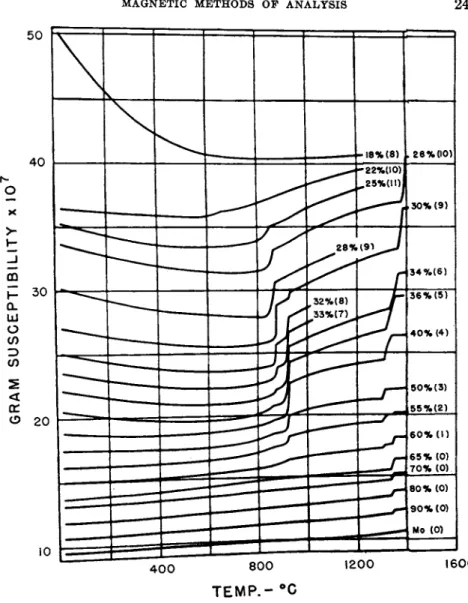
Another application of magnetic techniques is in t h e determination of phase diagrams or for detecting and following transformations in m a t e - rials. An extensive work on an alloy system (16) is shown in Fig. 13 which gives t h e susceptibility d a t a and Fig. 14 which presents t h e phase diagram obtained from it. A similar application t o t h e system Fe-S
MAGNETIC METHODS OP ANALYSIS 2 4 9
4 00 8 00 1200 1600
T E M P . - ° C
FIG. 13. Susceptibility vs. temperature in the Ni-Mo system.
(17), Fig. 15, shows how nicely solid solution in t h e compound F e S m a y be detected. T h e progress of a reaction a t t e m p e r a t u r e is illustrated in Fig. 16 where t h e susceptibility changes which occur during t h e precipi- tation of copper from a l u m i n u m are plotted (1).
9.4. Geological Applications
Magnetic measurements h a v e been used in a n u m b e r of geological studies. I n one case, similar s t r a t a below ground in adjacent areas, as
250 A. R. KAUFMANN
in a region of oil wells, are located b y susceptibility measurements on samples collected from various depths (30). D a t a on t h e orientation of t h e earth's field in p a s t ages h a v e been obtained b y measuring t h e orien
tation of magnetized impurities at various depths in t h e m u d of t h e ocean (18). Similar information has been obtained from sedimentary rocks (21).
9.5. Single Crystals
T h e orientation of single crystals of iron in t h e form of discs has been determined with an accuracy of a few degrees b y measuring t h e torque exerted b y a strong field whose direction lies in t h e plane of t h e specimen
1600 1400 1200 Ο ί Ο Ο Ο
I*
8 0 0φ Η 6 00
4 0 0 200
Ni 20 40 60 80 Mo W t . % Mo
FIG. 1 4 . Ni-Mo phase diagram as determined from susceptibility measurements.
(43). T h e m e t h o d is m u c h more rapid t h a n t h e s t a n d a r d x-ray technique and presumably can be applied t o other ferromagnetic single crystals.
M u c h information on t h e preferred orientation of crystals in a rolled sheet of ferromagnetic metal can be obtained b y t h e magnetic torque method. T h e spread of orientation about t h e fiber axis can be studied in this w a y (8).
9.6. Molecular Structure
Magnetic measurements provide a powerful m e t h o d for studying t h e electronic configuration of atoms, t h e degree of ionization of a t o m s in compounds and t h e structure of complex molecules a n d compounds.
This is based on t h e fact t h a t all magnetic phenomena (other t h a n nuclear effects) are due t o t h e electrons of atoms. An isolated electron has a definite magnetic m o m e n t (one Bohr magneton) and, in addition,
f—<~s= ^*-*r
^ ; . Ω
oc
/
OL+MMO mom\<X+M3M0-\^
β
V φ Λ
\
MAGNETIC METHODS OF ANALYSIS 251 electrons moving in closed orbits in a n a t o m produce magnetic effects just as does a microscopic electric current. T h e various electrons in an a t o m interact in a complicated w a y such t h a t t h e magnetic effects of t h e individual electrons cancel each other out whenever a shell of electrons is
χ 6 0 0 0 - 5 0 0 0 -
Region 1 v H max.=367 0
\ T - 2 0eC Jo
\ ισ»
\
fiC4 0 0 0 -
Phase 1 \ io>
1 \ |U
1 \ iO
ι \ Jo -
3 0 0 0 -
One ""One"
2 0 0 0 - ]Two Phas e Region \ j
1 0 0 0 -
| \ |
o-A 1 I '—1 r- ι — ι 1 1 1 1
I 12 1.4 1.6 1.8 2
FeS S - » - F e S 2
FIG. 15. Susceptibility in the iron-sulfur system.
completed. F o r this reason only t h e outer most electrons in incomplete shells contribute t o t h e p e r m a n e n t magnetic m o m e n t of a n a t o m .
W h e n a t o m s interact with each other as t h e y are brought together either in t h e pure elements or in compounds, t h e state of t h e outermost electrons will be altered a n d this shows u p as a change in magnetic
J-tfl ι ι ι ι I Μ
0,1 1 10
w w mo
Hours
FIG. 16. Susceptibility vs. aging time at various temperatures for quenched aluminum containing 5 % copper.
properties. A large variety of effects are possible ranging from normal paramagnetism through t h e t e m p e r a t u r e independent paramagnetism of most metals t o t h e ferromagnetic state. I n compound formation t h e exchange of electrons often leads t o completed electron shells for t h e
252 A. R. KAUFMANN
ions with a resultant loss of magnetic m o m e n t , t h u s leaving only a diamagnetic behavior. T h e magnetic m o m e n t of almost all atoms, b o t h neutral a n d ionized, can be calculated from known electronic configura- tions a n d a comparison of these various calculated values with t h e experi- mental quantities often leads t o definite information on t h e degree of ionization of atoms in various states (41).
All types of a t o m s experience a diamagnetic magnetization which, however, is often masked b y a stronger paramagnetic or ferromagnetic behavior. Diamagnetism is due t o a small change in t h e motion of the electrons moving around in an atom, which occurs as a result of t h e applied field. T h e change in motion is such t h a t a magnetization opposing t h e applied field is produced. Since all t h e electrons contribute to this behavior, changes in t h e outer electrons produce only small changes in diamagnetic m a t e r i a l Hence, it is possible t o approxi- mately compute t h e susceptibility of a diamagnetic compound just b y adding u p t h e known diamagnetic susceptibilities of t h e various a t o m s comprising t h e compound. Small correction quantities, known as Pascal's constants, need t o be added t o get complete agreement with experiment. I t is found t h a t for organic compounds t h e Pascal's con- stants have characteristic values for various molecular structures and, hence, susceptibility measurements on new substances can be used for determining t h e structure (27). T h e changes in bonding during poly- merization, for example, can be determined in this way.
B y means of magnetic measurements m u c h information has been obtained in recent years on t h e grouping of a t o m s into radicals in com- plex compounds, chiefly organic (28). These research methods should be of use not simply for scientific information b u t also for t h e chemical analyst who is trying t o develop new compounds.
I n recent years measurements of susceptibility have been carried out at radio a n d microwave frequencies using a weak microwave field at right angles t o a strong D . C . field which produces t h e magnetization.
Under these conditions it is found t h a t t h e specimen absorbs energy at certain resonance frequencies (15) a n d t h a t this phenomenon m a y be understood theoretically (20). T h e results are of interest in connection with physical theory b u t also could be of use t o t h e analyst since t h e energy absorption is determined b y t h e coupling between t h e magnetic m o m e n t and t h e other degrees of vibrational freedom of t h e atoms, and hence could yield information on t h e structure of liquids and solids.
9.7. Magnetic Titrations
A chemical reaction in which t h e magnetic m o m e n t of certain of the a t o m s or ions changes appreciably, m a y be followed b y means of mag-
MAGNETIC METHODS OF ANALYSIS 253 netic m e a s u r e m e n t s . I n t h i s w a y it is possible in m a n y cases t o tell when t h e reaction h a s gone t o completion a n d t h u s t o conclude, in t h e case of a k n o w n reaction, w h a t q u a n t i t y of one of t h e reacting substances was initially present. Conversely, if t h e a m o u n t s of reacting material are known, it is possible t o conclude w h a t t h e reaction h a s been t h r o u g h knowing t h e point a t which t h e reaction is complete. A n illustration of t h e l a t t e r procedure is shown in Fig. 17, where t h e change in susceptibility
16,000
12.000 Φ Ο
H 8,000 X
4,000
0
0 0.20 0.40 0.60 0.80 1.00 Ml. of 0 . 9 6 4/ K C N
FIG. 17. The magnetic titration of ferrihemoglobin with potassium cyanide at pH 6.75.
of a solution of ferrihemoglobin after various a d d i t o n s of K C N is plotted.
F r o m these d a t a it was concluded t h a t t h e reaction involved one cyanide per heme (12).
REFERENCES 1. Auer, Η., Z. Elektrochem. 45, 608 (1939).
2. Bates, L. F., Modern Magnetism, Cambridge, London, 1939, p. 6.
3. Bates, L. F., Modern Magnetism, Cambridge, London, 1939, p. 133.
4. Bates, L. F., Modern Magnetism, Cambridge, London, 1939, p. 70; Stoner, E. C , Magnetism and Matter, Methuen, London, 1934, p. 53.
5. Bitter, F., Rev. Set. Instruments 7, 482 (1936).
6. Bitter, F., Introduction to Ferromagnetism, McGraw-Hill, New York, 17 (1937).
7. Bitter, F., Introduction to Ferromagnetism, McGraw-Hill, New York, 194 (1937).
8. Bitter, F., Introduction to Ferromagnetism, McGraw-Hill, New York, 213 (1937).
9. Buehl, R., and Wulff, J., Rev. Sci. Instruments 9, 224 (1938).
10. Buehl, R., Holloman, H., Wulff, J., Trans. Am., Inst. Mining Met. Engrs. 140, 368 (1940).
11. Constant, F. W., Rev. Modern Phys. 17, 81 (1945); Bitter, F., and Kaufmann, A. R., Phys. Rev. 56, 1044 (1939).
12. Coryell, C , Stitt, F., Pauling, L., / . Am. Chem. Soc. 59, 633 (1937).
13. Dwight, Η. B., Am. Inst. Elec. Engrs., Technical Paper #42-27, Nov. 1941.
254 A. R. KAUFMANN 14. Foex, G., and Forrer, R., J. phys. radium 7, 180 (1926).
15. Griffiths, J. Η. E., Nature 158, 670 (1946).
16. Grube, G., and Winkler, Ο., Z. Elektrochem. 44, 423 (1938).
17. Haraldson, H., and Neuber, Α., Naturwissenschaften 24, 280 (1936).
18. Johnson, Ε. Α., and McNish, A. G., Terr. Magn. 43, 401 (1938).
19. Kaufmann, A. R., Rev. Sci. Instruments 9, 369 (1938).
20. Kittel, C., Phys. Rev. 71, 270 (1947).
21. Koenigsberger, J. G., Terr. Magn. 43, 119 and 299 (1938).
22. Leeds and Northrup Co. Notebook # 2 , Philadelphia, 1930, p. 32.
23. McKeehan, L. W., Rev. Sci. Instruments 5, 265 (1934).
24. Page, L., and Adams, N., Principles of Electricity, Van Nostrand, New York, 1934, p. 234.
25. Page, L., and Adams, N., Principles of Electricity, Van Nostrand, New York, 1934, p. 407; Bates, L. F., Modern Magnetism, Cambridge, London, 1939, p. 82.
26. Pauling, L., Wood, R. E., and Sturdivant, J. H., J. Am. Chem. Soc. 68, 795 (1946).
27. Selwood, P. W., Magnetochemistry, Interscience, New York, 1943, p. 51.
28. Selwood, P. W., Magnetochemistry, Interscience, New Yqrk, 1943, p. 116.
Weissberger, Α., Physical Methods of Organic Chemistry II, Interscience, New York, 1233 (1946).
29. Selwood, P. W., Magnetochemistry, Interscience, New York, 236 (1943).
30. Selwood, P. W., Magnetochemistry, Interscience, New York, 1943, p. 264.
31. Shuddemagen, C , Phys. Rev. 31, 165 (1910); Wurschmidt, J., Z. Physik 19, 388 (1923).
32. Spooner, T., Properties and Testing of Magnetic Materials, McGraw-Hill, New York, 1927, p. 231.
33. Spooner, T., Properties and Testing of Magnetic Materials, McGraw-Hill, New York, 1927, p. 302.
34. Starling, S. G., Electricity and Magnetism, Longman-Green, London, 1930, pp. 256 and 273.
35. Starr, C , Phys. Rev. 60, 245 (1941).
36. Stoner, E. C , Magnetism and Matter, Methuen, London, 1934, p. 39; Ewing, J. Α., Magnetic Induction in Iron and Other Metals, London, 1900, p. 24.
37. Stoner, E. C , Magnetism and Matter, Methuen, London, 1934, p. 57.
38. Stoner, E. C , Magnetism and Matter, Methuen, London, 1934, p. 60.
39. Stoner, E. C , Magnetism and Matter, Methuen, London, 1934, p. 70; Bates, L. F., Modern Magnetism, Cambridge, London, 1939, p. 91.
40. Stoner, E. C , Magnetism and Matter, Methuen, London, 1934, p. 251.
41. Stoner, E. C , Magnetism and Matter, Methuen, London, 1934, p. 310.
42. Sucksmith, W. Potter, H. and Broadway, L. Proc. Roy. Soc. London A117, 481 (1928).
43. Tarasov, L. P., and Bitter, F., Phys. Rev. 52, 353 (1937).
44. Weiss, P., and Onnes, K., J. phys. radium 9, 555 (1910).