2 Stability of the equilibria and local Hopf bifurcation

Hopf bifurcation analysis in a

neutral predator–prey model with age structure in prey

Daifeng Duan, Qiuhua Fan and Yuxiao Guo

Department of Mathematics, Harbin Institute of Technology, Weihai, Shandong, 264209, P.R. China Received 20 November 2018, appeared 28 April 2019

Communicated by Hans-Otto Walther

Abstract.We show a detailed study on the dynamics of a neutral delay differential pop- ulation model with age structure in the prey species. By selecting the mature delay as a bifurcation parameter, we obtain the stability and Hopf bifurcations of the coexistence equilibrium. Moreover, by computing the normal form on the center manifold, we give the formulas determining the stability of periodic solutions and the direction of Hopf bifurcation. Finally, we give some numerical simulations to support and strengthen the theoretical results.

Keywords: predator–prey, neutral type, age structure, Hopf bifurcation, delay.

2010 Mathematics Subject Classification: 37G15, 34K40.

1 Introduction

In recent years, neutral-type differential equations have been applied extensively in mathe- matical biologies and population dynamics [1,3,5], and their dynamical behaviors are usually very complex. In this paper we will consider the neutral delay differential equation with age structure as follows:

V˙(t)−b₂e^−µ0τV˙(t−τ) = b₁e^{−βV(t−τ)}+b₂µ₁

e^−µ0τV(t−τ)−µ₁V(t), (1.1) whereV(t)denotes the number of mature individuals in the population at timet,b₁andb₂are the birth rate and the maximum possible per capita egg production rate, respectively. µ₀ and µ₁ are the per capita mortality rate of the immature population and the adults, respectively.

τis the generation time and 1/βis the population size at which the whole population repro- duces at its maximum rate. One can derive this model (see [3]), from a structured population model foru(t,a)(the population density at timetand agea) as follows,

∂tu(t,a) +∂au(t,a) =−µ(a)u(t,a), with the death rate

µ(a) = (

µ₁, a>τ, µ₀, a<τ.

BCorresponding author. Email: gyx@hit.edu.cn

Then the total population of the mature individuals is V(t) = R_∞

τ u(t,a)da which fulfills Eq. (1.1). For more details on the derivation of (1.1), we refer the readers to [3].

By regarding V(t) as the prey population size, we incorporate a predation term g(V(t))U(t)into (1.1) to obtain the following general neutral prey-predator model:

(U˙(t) =−d₁U(t) +αg(V(t))U(t),

V˙(t)−b2e^−µ0τV˙(t−τ) = (b₁e^{−βV(t−τ)}+b2µ₁)e^−µ0τV(t−τ)−µ₁V(t)−cg(V(t))U(t). (1.2) Here the predator populationU(t)consume mature populationV(t)as food source,g:R+ → R+ is the functional response of predators, α represents the conversion rate from prey to predator,cis the per capita capturing rate of prey by a predator per unit time. For the case of linear functional responseg(V(t)) =V(t), reducing the model (1.2) to

(U˙(t) =−d₁U(t) +αU(t)V(t),

V˙(t)−b₂e^−µ0τV˙(t−τ) = (b₁e^{−βV(t−τ)}+b₂µ₁)e^−µ0τV(t−τ)−µ₁V(t)−cU(t)V(t). (1.3) There are many research findings of predator-prey model similar to Eq. (1.3) withb2 =0, i.e., in the absence of neutral delay effect, see [6,12,17,18]. For those models with neutral delay, Pielou [16] studied the effect of time delay in the population systems. Kuang [13] investi- gated a logistic model with the neutral term by introducing a time delay and obtained some sufficient conditions to ensure the local asymptotic stability of the positive equilibrium. In addition, there are few results about the delay neutral equation with age structure. Under as- sumption 0<b2<1, system (1.3) can be written as an abstract ordinary differential equation in suitable phase space by the theory on the decomposition of the phase space [8,9]. Com- pared with a predator-prey model without neutral delay [11,15,21,22], we find neutral delay may easily induce bifurcations. We obtain the above results by analyzing the characteristic equation and the normal forms near Hopf bifurcations.

This paper is organized as follows. In Section 2, we give the stability analysis and bi- furcation results about system (1.3). We find Hopf bifurcation occurs when the delay passes through some critical values. In Section 3, we offer algorithms for determining the direction of Hopf bifurcation and the stability of bifurcating periodic solutions by using the normal form method and the center manifold theory. In Section 4, we carry out some numerical simulations to support our results.

2 Stability of the equilibria and local Hopf bifurcation

In this section, we mainly analyze the stability of positive equilibrium in the cases ofτ=0 and τ>0. Regarding the stability and bifurcation of delay equation (1.3), the distribution analysis of roots of the characteristic equation plays an important role. Throughout this paper, we assume 0< b₂ <1 such that the neutral part of (1.1) defines a stable D-operator (see [8]). The equilibria of system (1.3) are the roots of the following equations:







(−d₁+αV)U=0, h

(b₁e^−βV+b₂µ₁)_e^−µ0τ−µ₁−cUi V =_0.

Then system (1.3) has three nonnegative equilibrium points:

(i) E₀= (_{0, 0}), which corresponds to the total extinction of the predator and prey;

(ii) E₁ = 0,¹_βln_µ ^b1

1(e^µ0τ−b2)

, which corresponds to the extinction of predator. The boundary equilibrium pointE₁ exists if and only ifτ< ¹

µ0ln^b1+_µ^b2µ1

1 ;

(iii) The interior equilibrium point E^∗ = (u^∗,v^∗), which corresponds to the coexistence state of prey and predator, and

u^∗ = ¹ c

b₁e^−βdα1 +b₂µ₁

e^−µ0τ− ^µ1

c , v^∗ = ^d1 α. E^∗ exists whenτ < τ_max := ¹

µ0ln^b1e−βd1/_µ^α+b2µ1

1 . The dynamics of the predator-free equilibrium E₁ has been investigated in a previous study in [5]. Biologically speaking, for model (1.3) we are interested to study the stability behavior of the interior equilibrium point E^∗. We first transform E^∗ = (u^∗,v^∗) of (1.3) to the origin via the translation u(t) = U(t)−u^∗ and v(t) =V(t)−v^∗, then the linearization of system (1.3) around the origin takes the form

(u˙(t) =αu^∗v(t),

v˙(t)−b2e^−µ0τv˙(t−τ) =−cv^∗u(t)−(µ₁+cu^∗)v(t) +a₁e^−µ0τv(t−τ), (2.1) where a₁ = (1−βv^∗)b₁e^−βv∗+b₂µ₁. The characteristic equation of (2.1) is

λ²+ (µ₁+cu^∗)λ+cαu^∗v^∗−(b₂λ²+a₁λ)_e^−µ0τ_e^−λτ =_{0. (2.2)} This is a characteristic equation with coefficients depending on time delay, so we employ the method in [2], rewrite (2.2) in the general form

P(λ,τ) +Q(λ,τ)e^−λτ =0, (2.3) where P(λ,τ) := λ²+ (µ₁+cu^∗)λ+cαu^∗v^∗, Q(λ,τ):= −(b₂λ²+a₁λ)e^−µ0τ. Forτ = 0, (2.3) becomes

(1−b2)λ²+b₁βv^∗e^−βv∗λ+cαu^∗v^∗ =0.

Obviously, we have the following lemma.

Lemma 2.1. Whenτ=0, the positive equilibrium E^∗of Eq.(1.3)is asymptotically stable.

When τ > 0, the distribution of the roots of the exponential polynomial equation with delay dependent parameters could not be analyzed in the usual way. Therefore, we introduce the geometric criterion established by Beretta and Kuang [2] (see also [14]). Firstly, we need to prove the following statements in order to discuss the distribution of the roots of (2.3) whose coefficients contain the delayτ.

Theorem 2.2. For system (2.3), the following geometric stability switch criterions (i)–(v) are estab- lished.

(i) P(0,τ) +Q(0,τ)6=0,∀τ∈_R+;

(ii) P(iω,τ) +Q(iω,τ)6=0,∀ω∈ _R,∀τ∈ _R+; (iii) lim supn

Q(λ,τ) P(λ,τ)

:|λ| →_{∞, Re}λ≥0o

<1,∀τ∈_R+;

(iv) F(ω,τ):=|P(iω,τ)|²− |Q(iω,τ)|² for eachτhas at most a finite number of real zeros;

(v) Each positive root ω(τ)of F(_ω,τ) =₀is continuous and differentiable inτwhenever it exists.

Proof. Obviously, by Eq. (2.3) we obtain P(0,τ) +Q(0,τ) =cαu^∗v^∗ >0,

P(iω,τ) +Q(iω,τ) =iωb₁βv^∗e^−µ0τe^−βv∗+ (b₂e^−µ0τ−1)ω²+cαu^∗v^∗ 6=0, thus the statements (i) and (ii) are established. In fact,

|λlim|→_∞

Q(λ,τ) P(λ,τ)

=b₂e^−µ0τ <1,

therefore (iii) holds true. Notice thatF(ω,τ)takes the following expression F(ω,τ) = 1−b₂²e^−2µ0τ

ω⁴+^h(µ₁+cu^∗)²−2cαu^∗v^∗−a²₁e^−2µ0τi

ω²+ (cαu^∗v^∗)². For each τ, F(ω,τ) = 0 has at most a finite number of real zeros. The statement (v) is also satisfied by the implicit function theorem.

Lemma 2.3(see [14]). Based on Theorem2.2, the following conclusions are valid.

(a) When F(ω,τ) =0has no positive roots, there is no stability switch.

(b) When F(ω,τ) = 0 has at least one positive root and each of them is simple, a finite number of stability switches may occur with the increase ofτ.

Remark 2.4. Claim (i) implies thatλ=0 is not a characteristic root of (2.3) and (ii) implies that P(_λ,τ)_andQ(_λ,τ)have no identical imaginary roots. Claim (iii) guarantees that the roots of the equation (2.3) with non-negative real parts are uniformly bounded. Claim (iv) guarantees that the equation (2.3) has at most a finite number of imaginary roots for the givenτ, that is, there are only finite times for roots to cross the imaginary axis with the change ofτ. Claim (v) is used to compute the derivative of the imaginary roots with respect toτ.

Combined with the conclusion of Lemma2.3, we will study the existence of Hopf bifur- cation for system (1.3). Assume that λ = iω (ω > 0) is the pure imaginary root of (2.2), then

−ω²+iω(µ₁+cu^∗) +cαu^∗v^∗+ (b2ω²−iωa₁)e^−µ0τ(cosωτ−isinωτ) =0.

Separating the real and imaginary parts, we get







sinωτ = ^cαu∗v∗a₍^{1−a1ω2+b2ω2(µ1+cu∗)}

a²₁ω+b²₂ω³)e^−µ0τ =S(τ), cosωτ =−^cαu∗v∗b₍^{2ω−b2ω3−a1ω(µ1+cu∗)}

a²₁ω+b²₂ω³)e^−µ0τ =C(τ), which leads to

F(ω,τ) =0. (2.4)

Letz=ω², then (2.4) becomes

1−b₂²e^−2µ0τ

z²+Az+ (cαu^∗v^∗)² =0, (2.5) where A= (µ₁+cu^∗)²−2cαu^∗v^∗−a²₁e^−2µ0τ. Notice that 1−b²₂e^−2µ0τ >_0, (cαu^∗v^∗)² >_0.

Thus, we further make the following assumptions:

(H1) A<0,

(H2) A+2cαu^∗v^∗(1−b²₂e^−2µ0τ)^1/2 <0,

then there exist two positive real rootsω±(τ)of (2.5),

ω±(τ) =





−A±^qA²−4(1−b²₂e^−2µ0τ)(cαu^∗v^∗)² 2(1−b₂²e^−2µ0τ)





1/2

. Set

I ={τ|A<0,A²−4(1−b²₂e^−2µ0τ)(cαu^∗v^∗)²>0,τ∈ (0, ˆτ]}.

When I is nonempty, forτ ∈ I, there existω+(τ)> 0,ω−(τ)> 0 such that F(ω,τ) = 0. For τ∈ I,θ(τ)∈(0, 2π]is defined by







sinθ(τ) = ^cαu∗v∗a₍^{1−a1ω2+b2ω2(µ1+cu∗)}

a²₁ω+b²₂ω³)e^−µ0τ , cosθ(τ) =−^cαu∗v∗b₍^{2ω−b2ω3−a1ω(µ1+cu∗)}

a²₁ω+b²₂ω³)e^−µ0τ ,

then we have ω(τ)τ = θ(τ) +2nπ. Hence, iω is a purely imaginary root of Eq. (2.2) if and only if τis a zero of the functionS_n(τ), defined by

S_n(τ) =τ−^θ(τ) +2nπ

ω(τ) ^{, τ}∈ I, n∈_N0. (2.6)

We list the basic results to show the occurrence of Hopf bifurcation in [2] as follows.

Lemma 2.5. Assume thatω(τ)is a positive real root of Eq.(2.4)and at someτ_k ∈ I, Sn(τ_k) =0, for some n ∈_N0.

Whenτ =τ_k,λ= ±iω(τ_k)is a pair of conjugate purely imaginary roots of Eq.(2.3), and ifδ(τ_k)>

0(<0), the roots corresponding to the conjugate purely imaginary roots cross the imaginary axis from left (right) to right (left), where

δ(τ_k) =sign

dReλ dτ

λ=iω(τ_k)

=sign

F_ω⁰ (ω(τ_k),τ_k) sign

dSn(τ) dτ

τ=τ_k

.

The next theorem is concerned with the stability for system (1.3) and the Hopf bifurcation.

Theorem 2.6. For some m = 1, 2, . . ., assume that every S_k(τ) (k = 0, 1, . . . ,m−1) defined by Eq.(2.6)has exactly two rootsτ=τ_kandτ_2m−1−kwithτ0 <τ₁ <· · · <τ2m−1, and that S_k⁰(τ_k)>0 and S⁰_k(τ_2m−1−k) < 0. Further assume S_k(τ) has no roots on {τ : τ ≥ 0}for any k ≥ m, then we have

(i) whenτ∈[0,τ₀)∪(τ_2m−1, ˆτ), the roots of the characteristic equation(2.2)have strictly negative real part and the positive equilibrium of Eq.(1.3)is asymptotically stable;

(ii) whenτ∈ (τ_k,τ_k+1)∪(τ_2m−2−k,τ_2m−1−k), k =0, 1, . . . ,m−1, the characteristic equation(2.2) has exactly k+1pairs of roots with the positive real part, and the positive equilibrium of Eq.(1.3) is unstable.

(iii) whenτ=τ_k,k=0, 1, . . . , 2m−1, the characteristic equation(2.2)has a pair of imaginary roots

±iω_k withω_k = ω_2m−1−k, and Eq.(1.3)undergoes a Hopf bifurcation at the positive equilibrium E^∗.

Remark 2.7. The stability of the positive equilibrium and the existence of Hopf bifurcation for system (1.3) have been investigated by analyzing the distribution of eigenvalues. It is notewor- thy that (2.3) is an exponential polynomial equation with time delay in coefficients. In order to discuss the distribution of the roots of such equations, it is necessary to use the geometric criterion in [2] for the existence of purely imaginary roots, which is shown in Theorem 2.2 above.

3 Stability and direction of Hopf bifurcation

In this section, we will study the direction of Hopf bifurcation and the stability of bifurcating periodic solutions of model (1.3). The method to compute normal forms restricted on center manifolds is due to [4,7,19,20]. For simplicity, letu(t) = U(τt)−u^∗,v(t) = V(τt)−v^∗, and τ=τ+µ(τ∈ {τ0,τ₁, . . . ,τ2m−1}). System (1.3) is written as











˙

u(t) =τ

−d₁(u^∗+u(t)) +α(u^∗+u(t))(v^∗+v(t)),

˙

v(t)−b2e^−µ0τv˙(t−1) =τ

(b₁e^{−β(v∗+v(t−1))}+b2µ₁)e^−µ0τ(v^∗+v(t−1))

−τµ₁(v^∗+v(t))−τc(u^∗+u(t))(v^∗+v(t)).

(3.1)

DenoteC=C([−1, 0],R²), then rewrite Eq. (3.1) as d

dt[DXt] =L0Xt+ (Lµ−L0)Xt+F(Xt,µ), where

Dφ=

ϕ₁(0)

ϕ₂(0)−b2e^−µ0τϕ₂(−1)

, Lµφ= (τ+µ)(B₁φ(0) +B₂φ(−1)), and

F(φ,µ) = (τ+µ) ^αϕ1(0)ϕ₂(0)

−cϕ₁(0)ϕ₂(0) +b₁βe^{−(βv∗+µ0τ)}h

βv^∗

2 −1+ (^β₂− ^β2₆^v∗)ϕ₂(−1)ⁱϕ²₂(−1)

!

forφ= (ϕ₁,ϕ₂)∈C, and B₁ =

0 αu^∗

−cv^∗ −µ₁−cu^∗

, B₂=

0 0 0 a₁e^−µ0τ

. Choosing

µ(θ) =

(D₁, θ= −1,

D₂, θ∈ (−1, 0], and η(µ,θ) =











−(τ+µ)_B2, θ =−1, 0, θ ∈(−1, 0), (τ+µ)B₁, θ =0, where

D₁=

0 0 0 −b₂e^−µ0τ

, D₂=

0 0 0 0

,

then we have

Dφ=φ(0)−

Z ₀

−1dµ(θ)φ(θ), L₀φ=

Z ₀

−1dη(0,θ)φ(θ). Define

A(µ)φ=

(dφ(θ)/dθ, θ ∈[−1, 0), φ⁰(₀)−Dφ⁰(θ) +L_µφ, θ =₀ and

R(µ)φ=

(0, θ ∈[−1, 0), F(φ,µ), θ =0.

Then (3.1) can be written as

X˙_t = A(µ)X_t+R(µ)X_t, (3.2) where X(t) = (u(t),v(t))^T, X_t= X(t+θ),θ ∈[−1, 0]. Clearly, (3.2) is an abstract ODE on the phase space BC(see [19]), where

BC =φ:[−1, 0]→_R², φis continuous on[−1, 0)_{, and limθ→0}φ(θ)_{exists .} The adjoint operator A^∗ is defined byA^∗ψ= −^dψ_ds with domain

D(A^∗) =

ψ∈C^∗= C([0, 1],R²): dψ

ds ∈C^∗;Ddψ

ds =−Lψ

.

Applying the formal adjoint theory in [8], we decompose C by Λ as C = P⊕Q, where P = span{_Φ(θ)}and choose a basis Ψ for the adjoint space P^∗, such thath_Ψ,Φi = 1, where h·,·iis the bilinear form onC^∗×Cdefined by

(ψ,φ) =ψ^¯(0)φ(0)−

Z ₀

−1d Z _θ

0

ψ¯(θ−α)d[µ(α)]

φ(θ)−

Z ₀

−1

Z _θ

0

ψ¯(ξ−θ)d[η(0,θ)]φ(ξ)dξ.

Let q∈ Candq^∗ ∈C^∗ be the eigenvectors of A(0)andA^∗ corresponding to eigenvaluesiωτ¯ and−iωτ, respectively. Then we have¯

q(θ) = (1,q₂)^Te^iωτθ¯ , θ ∈[−1, 0], q^∗(s) =D(1,q^∗₂)e^iωτs¯ , s∈[0, 1], where

q₂ = ^iω

αu^∗, q^∗₂ = ^iω

cv^∗, D= ¹

1+q¯^∗₂q₂+τ¯q¯^∗₂q₂a₁e^−µ0τe^−iωτ¯+q¯^∗₂q₂b₂e^−µ0τe^−iωτ¯. Using a computation process similar to [10], we compute the center manifold C₀ at µ = 0.

Define

z(t) =hq^∗,uti,w(t,θ) =ut(θ)−2 Re{z(t)q(θ)}. On the center manifoldC₀ we havew(t,θ) =w(z(t), ¯z(t),θ), where

w(z(t), ¯z(t),θ) =w₂₀(θ)^z

2

2 +w₁₁(θ)zz¯+w₀₂(θ)^z¯

2

2 +· · · ,

zand ¯z are local coordinates for center manifold C₀ in the direction ofq^∗ and ¯q^∗. Notice that wis real ifu_t is real.

For solutionu_tin C₀of Eq. (3.1), sinceµ=0,

˙

z(t) =iωτz¯ +hq^∗(θ),f(w+2Re{z(t)q(θ)})i

=iωτz¯ +q¯^∗f(w(z, ¯z, 0) +2Re{z(t)q(0)})

=iωτz¯ +q¯^∗f₀(z, ¯z),

(3.3)

with f₀(z, ¯z) = f_z2z²

2 + f_zz¯zz¯+f_z¯2z¯²

2 + f_z2z¯z²z¯

2 +· · · . Eq. (3.3) can be rewritten in the abbreviated form as

˙

z(t) =iωτz¯ (t) +g(z, ¯z), (3.4) where

g(z, ¯z) = g₂₀z²

2 +g₁₁zz¯+g₀₂z¯²

2 +g₂₁z²z¯

2 +· · · . (3.5) By (3.2) and (3.4), we have

˙

w= X^˙_t−zq˙ −z˙¯q¯

=

(Aw−2 Re{q¯^∗(0)f₀q(θ)}, θ∈ [−1, 0), Aw−2 Re{q¯^∗(0)f₀q(0)}+ f₀, θ=0,

def= Aw+H(z, ¯z,θ)_,

(3.6)

where H(z, ¯z,θ) = H₂₀(θ)^z₂² + H₁₁(θ)zz¯+H₀₂(θ)^z¯₂² +· · ·. Comparing the coefficients, we obtain

(A−2iωτI¯ )w₂₀(θ) =−H₂₀(θ), Aw₁₁(θ) =−H₁₁(θ), . . . Note that

q^∗(0) =D(1,q₂^∗), u(t) =z+z¯+w⁽¹⁾(z, ¯z, 0), v(t) =q₂z+q¯₂z¯+w⁽²⁾(z, ¯z, 0),

v(t−1) =q₂e^−iωτ¯z+q¯₂e^iωτ¯z¯+w⁽²⁾(z, ¯z,−1) where

w⁽¹⁾(z, ¯z, 0) =w⁽₂₀¹⁾(0)^z

2

2 +w⁽₁₁¹⁾(0)zz¯+w⁽₀₂¹⁾(0)^z¯

2

2 +· · · , w⁽²⁾(z, ¯z, 0) =w⁽₂₀²⁾(0)^z

2

2 +w⁽₁₁²⁾(0)zz¯+w⁽₀₂²⁾(0)^z¯

2

2 +· · · , w⁽²⁾(z, ¯z,−1) =w⁽₂₀²⁾(−1)^z

2

2 +w⁽₁₁²⁾(−1)zz¯+w₀₂⁽²⁾(−1)^z¯

2

2 +· · · . Comparing the coefficients with Eq. (3.5), we have

g₂₀=2Dτ¯

(α−q¯^∗₂c)q₂+q¯^∗₂q²₂b₁βe^−βv∗e^−µ0τ(βv^∗/2−1)e^−2iωτ¯ , g₁₁= Dτ¯

(α−q¯^∗₂c)(q2+q¯2) +2 ¯q^∗₂q2q¯2b₁βe^−βv∗e^−µ0τ(βv^∗/2−1), g₀₂=2Dτ¯

(α−q¯^∗₂c)q¯₂+q¯^∗₂q¯²₂b₁βe^−βv∗e^−µ0τ(βv^∗/2−₁)_e^2iωτ¯_, g₂₁=2Dτ¯

(α−q¯^∗₂c)(w⁽₂₀¹⁾(0)^q¯2 2 + ^w

(2) 20(0)

2 +w⁽₁₁²⁾(0) +w₁₁⁽¹⁾(0)q2) +q¯^∗₂b₁βe^−βv∗e^−µ0τ

(βv^∗/2−1)(2q₂w⁽₁₁²⁾(−1)e^−iωτ¯ +q¯₂w⁽₂₀²⁾(−1)e^iωτ¯) + (β/2−β²v^∗/6)3q²₂q¯₂e^−iωτ¯

.

We need to calculatew₂₀(θ)andw₁₁(θ). By (3.6), we have w₂₀(θ) = −g₂₀

iωτ¯ q(0)e^iωτθ¯ − ^g¯02

3iωτ¯q¯(0)e^−iωτθ¯ +E₁e^2iωτθ¯ , w₁₁(θ) = ^g11

iωτ¯q(₀)_e^iωτθ¯ − ^g¯11

iωτ¯q¯(₀)_e^−iωτθ¯ +E₂, where

E₁ = (2iωτId¯ ₂×2+2iωτD¯ ₁−τB¯ ₁−τB¯ ₂e^−2iωτ¯)⁻¹f_z2, E₂ =−τ¯⁻¹(B₁+B₂)⁻¹f_zz¯,

and

f_z² =2 ¯τ(αq2,−cq2+q²₂b₁βe^−βv∗e^−µ0τ(βv^∗/2−1)e^−2iωτ¯)^T,

f_zz¯ =τ¯(α(q₂+q¯₂),−c(q₂+q¯₂) +2q₂q¯₂b₁βe^−βv∗e^−µ0τ(βv^∗/2−1))^T. Consequently,g₂₁could be expressed explicitly. Denote

c₁(₀) = ⁱ 2wτ¯

g₁₁g₂₀−₂|g₁₁|²− |g₀₂|² 3

+ ^g21

2 , µ₂ = − ^Re(c₁(0))

Re(λ⁰(τ¯))^, β₂ =2 Re(c₁(0)).

According to the general results from [20], we have the following conclusion.

Theorem 3.1. µ₂ determines the direction of Hopf bifurcation: if µ₂ > 0 (< 0), then the bifurcat- ing periodic solutions are forward (backward); β₂ determines the stability of the bifurcation periodic solutions: the bifurcation periodic solutions are orbitally stable (unstable) on the center manifold if β₂ <0(>0).

4 Numerical simulation

In this section, we shall carry out the numerical simulation on system (1.3). We choose µ₀ =0.035, µ₁=0.03, d₁=0.2, b₁=5, b₂ =0.5, α=0.015, β=0.3, c=0.2.

For this set of parameter values, we observe that (H1) and (H2) hold, and τ_max = 36.2195.

The condition 0 ≤ τ < τ_max is used to guarantee the existence of positive equilibrium E^∗. In particular, τmax > 0 means the birth rate of the prey population is far greater than the death rate of the adults based on the biological mechanism. The conditions (H1) and (H2) hold in the case of τ ∈ [0,τ_max), which provides a possibility for periodic oscillation of system (1.3).

According to Theorem 2.6, we know m = 1, the graph of S0 versus τ shown in Figure 4.1.

One can find thatS₀ has two zeros, the first at the valueτ₀ = 5.4792, the second at the value τ₁ = 39.1335 (τ₁ > τ_max), withS⁰₀(τ₀)> 0 and S⁰₀(τ₁)< 0. The rest functionsS₁,S₂, . . . , have no roots. Notice that ¯τ = τ0, λ⁰(τ¯)can be easily calculated by Lemma2.5. According to the expressions ofc₁(0),µ₂ andβ₂ in Section3, we get

c₁(0) =−0.0787−1.8163i, µ₂=136.5534, β₂=−0.1574.

By the results to Theorem 3.1, the bifurcating periodic solutions of system (1.3) are for- ward sinceµ₂ >0. Besides, the bifurcation periodic solutions are orbitally stable sinceβ₂ <0.

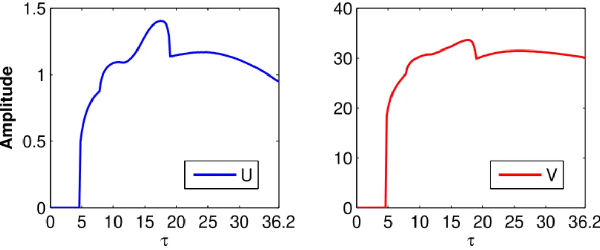
Therefore, when τ ∈ [0,τ₀), the positive equilibrium (u^∗,v^∗) of Eq. (1.3) is asymptotically stable; when τ ∈ (τ₀,τ_max), the positive equilibrium of Eq. (1.3) is unstable; when τ = τ₀ or τ = τ₁, Eq. (1.3) undergoes a Hopf bifurcation at the positive equilibrium. Furthermore, according to Theorem3.1, the Hopf bifurcation of Eq. (1.3) is supercritical, and the bifurcating periodic solution is asymptotically stable (see Figure 4.2). When τ ∈ [0, 36.2195), the cor- responding amplitude diagrams of the predator U and the prey V (see Figure 4.3) are also given. We can find that whenτ ∈ [0,τ₀), the amplitudes ofU and V are both zero. When τ∈(τ₀,τ_max), it will increase gradually, then decrease secondly.

0 5 10 15 20 25 30 35 40

−200

−150

−100

−50 0 50

τ

S n

τ_max

S0 S1 S2

Figure 4.1: The graph of functionsS0,S₁ andS2 forτ∈[0, ˆτ).

0 50 100 150 200 250 300

0 5 10 15

τ

U V

(a)

0 50 100 150 200 250 300

0 5 10 15 20 25 30

τ

U V

(b)

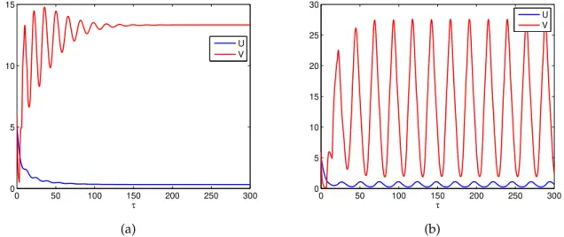
Figure 4.2: (a) The positive equilibrium of Eq. (1.3) is asymptotically stable whenτ = 3 < τ0. (b) A stable periodic solution bifurcating from the positive equilibrium whenτ=7>τ₀.

Remark 4.1. The positive equilibrium E^∗ exists when τ ∈ [_{0, 36.2195}). With the increase of

0 5 10 15 20 25 30 36.2 0

0.5 1 1.5

τ

Amplitude

U

0 5 10 15 20 25 30 36.2 0

10 20 30 40

τ

V

Figure 4.3: The amplitude ofUandVwhenτ∈[0, 36.2195).

τ, the periodic orbit oscillates near the positive equilibrium in (U,V) plane. The boundary equilibrium E₁ exists when τ ∈ [0, 146.2569). When τ > 36.2195, the positive equilibrium disappears and the amplitude periodic solution oscillates near E₁. The numerical simulation shows that the periodic solution will eventually oscillate periodically on theV-axis.

5 Conclusions

In this paper, we study a neutral predator-prey system with age structure in prey. Stability and Hopf bifurcation results about the inner equilibrium are obtained. From the theoretical analysis, one can find that neutral delay terms can alter the dynamics of the Lotka–Volterra system significantly.

Acknowledgments

The authors would like to express their thanks to the referees for their careful reading, helpful comments, and valuable suggestions. In addition, this work is supported by the National Natural Science Foundation of China (No. 11701120 and No. 11771109).

References

[1] E. Beretta, Y. Kuang, Convergence results in a well-known delayed predator–prey sys- tem, J. Math. Anal. Appl. 204(1996), No. 3, 840–853. https://doi.org/10.1006/jmaa.

1996.0471;MR1422776;Zbl 0876.92021

[2] E. Beretta, Y. Kuang, Geometric stability switch criteria in delay differential systems with delay dependent parameters,SIAM J. Math. Anal.33(2002), No. 5, 1144–1165.https:

//doi.org/10.1137/S0036141000376086;MR1897706;Zbl 1013.92034

[3] G. Bocharov, K. P. Hadeler, Structured population models, conservation laws, and delay equations,J. Differential Equations168(2000), No. 1, 212–237. https://doi.org/10.

1006/jdeq.2000.3885;MR1801352;Zbl 0972.34059

[4] J. Carr, Applications of centre manifold theory, Springer, New York, 1981. https://doi.

org/10.1007/978-1-4612-5929-9;MR0635782

[5] D. Duan, B. Niu, J. Wei, Local and global Hopf bifurcation in a neutral population model with age structure,Math. Method. Appl. Sci.(2019).https://doi.org/10.1002/mma.5689 [6] G. H. Erjaee, F. M. Dannan, Stability analysis of periodic solutions to the nonstan-

dard discretized model of the Lotka–Volterra predator–prey system, Internat J. Bifur- cat. Chaos. 14(2004), No. 12, 4301–4308. https://doi.org/10.1142/s0218127404011946;

MR2118652;Zbl 1089.34528

[7] T. Faria, L. Magalhães, Normal forms for retarded functional-differential equations with parameters and applications to Hopf bifurcation, J. Differential Equations122(1995), No. 2, 181–200.https://doi.org/10.1006/jdeq.1995.1144;MR1355888;Zbl 0836.34068 [8] J. K. Hale, S. M. VerduynLunel,Introduction to functional-differential equations, Springer-

Verlag, New York, 1993.https://doi.org/10.1007/978-1-4612-4342-7;MR1243878 [9] J. K. Hale, M. Weedermann, On perturbations of delay-differential equations with peri-

odic orbits,J. Differential Equations197(2004), No. 2, 219–246.https://doi.org/10.1016/

S0022-0396(02)00063-3;MR2034159

[10] B. Hassard, N. D. Kazarinoff, Y. Wan, Theory and applications of Hopf bifurcation, Cam- bridge Univ. Press, Cambridge, 1981.MR0603442;

[11] J. Huang, S. Ruan, J. Song, Bifurcations in a predator–prey system of Leslie type with generalized Holling type III functional response,J. Differential Equations257(2014), No. 6, 1721–1752.https://doi.org/10.1016/j.jde.2014.04.024;MR3227281;Zbl 1326.34082 [12] P. Kloeden, C. Pötzsche, Dynamics of modified predator–prey models, Internat J. Bi-

furcat. Chaos.20(2010), No. 9, 2657–2669.https://doi.org/10.1142/S0218127410027271;

MR2738725

[13] Y. Kuang, On neutral delay logistic Gause-type predator–prey systems,Dyn. Stab. Syst.

6(1991), No. 2, 173–189. https://doi.org/10.1080/02681119108806114; MR1113116;

Zbl 0728.92016

[14] Y. Kuang, Delay differential equations with applications in population dynamics, Academic Press, Boston, 1993.MR1218880

[15] S. Kundu, S. Maitra, Dynamics of a delayed predator–prey system with stage structure and cooperation for preys, Chaos. Soliton. Fractal.114(2018), 453–460. https://doi.org/

10.1016/j.chaos.2018.07.013;MR3856667

[16] E. C. Pielou,Mathematical ecology, Wiley, New York, 1977.MR0434494

[17] H. Shu, L. Wang, J. Wu, Global dynamics of Nicholson’s blowflies equation revisited:

Onset and termination of nonlinear oscillations,J. Differential Equations255(2013), No. 9, 2565–2586.https://doi.org/10.1016/j.jde.2013.06.020;MR3090069;Zbl 1301.34107 [18] Y. Song, J. Wei, Local Hopf bifurcation and global periodic solutions in a delayed

predator–prey system, J. Math. Anal. Appl.301(2005), No. 1, 1–21.https://doi.org/10.

1016/j.jmaa.2004.06.056;MR2105917

[19] C. Wang, J. Wei, Normal forms for NFDEs with parameters and application to the lossless transmission line,Nonlinear Dynam.52(2008), No. 3, 199–206.https://doi.org/10.1007/

s11071-007-9271-9;MR2390855;Zbl 1187.34094

[20] S. Wiggins, Introduction to applied nonlinear dynamical systems and chaos, Springer-Verlag, New York, 1990.MR1056699

[21] A. M. Yousef, S. M. Salman, A. A. Elsadany, Stability and bifurcation analysis of a delayed discrete predator–prey model,Internat J. Bifurcat. Chaos.28(2018), No. 9, 1850116.

https://doi.org/10.1142/S021812741850116X;MR3851295;Zbl 1401.39021

[22] G. Zhu, J. Wei, Global stability and bifurcation analysis of a delayed predator–prey system with prey immigration, Electron. J. Qual. Theory Differ. Equ. 2016, No. 13, 1–20.

https://doi.org/10.14232/ejqtde.2016.1.13;MR3478754;Zbl 1363.34313