E xplosive diversification events, with intermittent periods of relatively little change, have generated uneven patterns of spe- cies richness across the tree of life. Although rapid radiations have been inferred in many clades1–5, few examples exist for fungi, in part because of their limited fossil record, and the lack of compre- hensive phylogenies. Advances in modelling the evolutionary pro- cess now allow such inferences to be made from phylogenetic trees.
Studies of diversification of mushroom-forming fungi have focused on individual clades
6–9, yielding hypotheses on ecological oppor- tunities
6, the evolution of mutualistic lifestyle
7,10and fruiting body morphologies
6,11as drivers of adaptive evolution in fungi. However, these inferences, based on specific clades, remained untested across larger phylogenetic scales. Fruiting bodies provide support and protection for developing spores, which probably represents a driv- ing force for increasingly more efficient morphologies
12. Ancestral fruiting bodies of the Agaricomycotina were probably crust-like,
‘resupinate’ forms
13,14, which then evolved into increasingly more
complex forms, including derived ‘pileate-stipitate’ types, which are differentiated into a cap, stipe and hymenophore (spore-bearing surface). Pileate-stipitate forms have arisen repeatedly from simpler morphologies (for example, resupinate or coral-like) during evolu- tion
12,13,15and dominate extant agaricomycete diversity (>21,000 described species
16), but how this diversity arose, what explains the dominance of pileate-stipitate species in the class and whether fruit- ing body morphology impacts diversification rates (for example, as a key innovation) are not known.
Results and discussion
We investigated broad patterns of diversification in Agaricomycetes using a phylogenetic comparative approach and generated a highly comprehensive phylogeny of the group, comprising 5,284 spe- cies (Fig. 1). Our dataset represents around 26% of described Agaricomycetes, a notably high sampling density for any fun- gal group. Our inferences of phylogenetic trees combine a robust
Megaphylogeny resolves global patterns of mushroom evolution
Torda Varga
1, Krisztina Krizsán
1, Csenge Földi
1, Bálint Dima
2, Marisol Sánchez-García
3, Santiago Sánchez-Ramírez
4, Gergely J. Szöllősi
5, János G. Szarkándi
6, Viktor Papp
7,
László Albert
8, William Andreopoulos
9, Claudio Angelini
10,11, Vladimír Antonín
12, Kerrie W. Barry
9, Neale L. Bougher
13, Peter Buchanan
14, Bart Buyck
15, Viktória Bense
1, Pam Catcheside
16,
Mansi Chovatia
9, Jerry Cooper
17, Wolfgang Dämon
18, Dennis Desjardin
19, Péter Finy
20, József Geml
21, Sajeet Haridas
9, Karen Hughes
22, Alfredo Justo
3, Dariusz Karasiński
23, Ivona Kautmanova
24,
Brigitta Kiss
1, Sándor Kocsubé
6, Heikki Kotiranta
25, Kurt M. LaButti
9, Bernardo E. Lechner
26, Kare Liimatainen
27, Anna Lipzen
9, Zoltán Lukács
28, Sirma Mihaltcheva
9, Louis N. Morgado
21,41, Tuula Niskanen
27, Machiel E. Noordeloos
21, Robin A. Ohm
29, Beatriz Ortiz-Santana
30, Clark Ovrebo
31, Nikolett Rácz
6, Robert Riley
9, Anton Savchenko
32,42, Anton Shiryaev
33, Karl Soop
34, Viacheslav Spirin
32, Csilla Szebenyi
6,43, Michal Tomšovský
35, Rodham E. Tulloss
36,37, Jessie Uehling
38, Igor V. Grigoriev
9,39, Csaba Vágvölgyi
6, Tamás Papp
6,43, Francis M. Martin
40, Otto Miettinen
32, David S. Hibbett
3and László G. Nagy
1*
Mushroom-forming fungi (Agaricomycetes) have the greatest morphological diversity and complexity of any group of fungi.
They have radiated into most niches and fulfil diverse roles in the ecosystem, including wood decomposers, pathogens or mycorrhizal mutualists. Despite the importance of mushroom-forming fungi, large-scale patterns of their evolutionary his- tory are poorly known, in part due to the lack of a comprehensive and dated molecular phylogeny. Here, using multigene and genome-based data, we assemble a 5,284-species phylogenetic tree and infer ages and broad patterns of speciation/extinction and morphological innovation in mushroom-forming fungi. Agaricomycetes started a rapid class-wide radiation in the Jurassic, coinciding with the spread of (sub)tropical coniferous forests and a warming climate. A possible mass extinction, several clade-specific adaptive radiations and morphological diversification of fruiting bodies followed during the Cretaceous and the Paleogene, convergently giving rise to the classic toadstool morphology, with a cap, stalk and gills (pileate-stipitate morphol- ogy). This morphology is associated with increased rates of lineage diversification, suggesting it represents a key innovation in the evolution of mushroom-forming fungi. The increase in mushroom diversity started during the Mesozoic-Cenozoic radiation event, an era of humid climate when terrestrial communities dominated by gymnosperms and reptiles were also expanding.
A full list of affiliations appears at the end of the paper.
genome-based backbone phylogeny of 104 species (650 genes, 141,951 amino acid characters, see Supplementary Figs. 1–3, Supplementary Table 1 and Supplementary Notes 1 and 2) with sequence data from up to three nuclear loci for 5,284 taxa (large subunit (LSU) rRNA, rpb2, ef-1a, 5,737 characters). New sequence data were generated for 1,222 species (Supplementary Note 2 and Supplementary Data 1), including nine new genomes of phyloge-
netically key taxa (Supplementary Note 3). The phylogenetic tree topology is largely congruent with previously published clade- specific phylogenies and resolves 21 orders of Agaricomycetes plus Dacrymycetes and Tremellomycetes as outgroups. Most of the nodes received strong bootstrap support, but we also identi- fied nodes that require more scrutiny and probably denser taxon sampling to be resolved with certainty (for a detailed genome-based
Car
b.
Perm
ian
Perm
iann
Perm
ia
Car
b.
Car
b
Agaricomycetidae 191–176 Myr
Polyporales (bracket fungi) Agaricaceae
(button mushrooms)
Boletales Hymenochaetales
Phallomycetidae Cantharellales
Dacrymycetes Tremellomycetes
Russulales Psathyrellaceae
(inky caps)
Omphalotaceae (Shiitake and allies)
Marasmiaceae
Pleurotaceae (oyster mushrooms)
Hygrophoraceae (waxcaps and allies) Entolomataceae Cortinarius
Lycoperdaceae (true puffballs)
Amanitaceae (death cap and allies)
Inocybaceae Strophariaceae
Agaricales 182–156 Myr
–0.16 0.10 0.15 0.51
Net diversification rate Angiosperm
Gymnosperm Substrate
4 6 8 10 no. of trees with shift
Auriculariales Trechisporales
Jaapiales Corticiales Gloeophyllales
Amylocorticiales Atheliales Lepidostromatales Stereopsidales Thelephorales
Tria
ssic
Jurassic
Cretace
ous
Paleogene
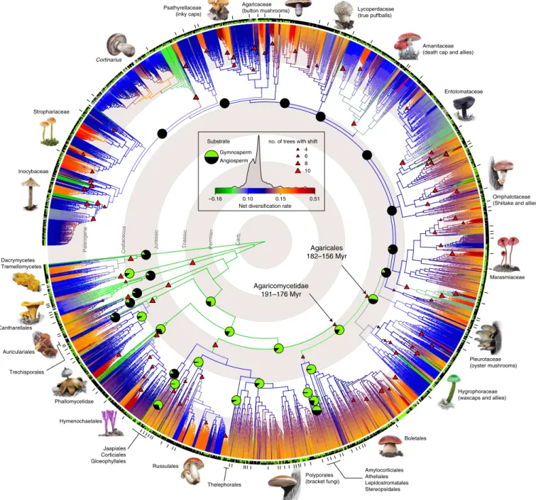
Fig. 1 | Phylogenetic relationships and diversification across 5,284 mushroom-forming fungi. One of the 245 analysed maximum-likelihood trees was randomly chosen and visualized. Trees were inferred from nrLSU, rpb2, ef1-a sequences with a phylogenomic backbone constraint of deep nodes. Branches are coloured by net diversification (speciation minus extinction) rate inferred in Bayesian Analysis of Macroevolutionary Mixtures (BAMM). Warmer colours denote a higher rate of diversification. Significant shifts in diversification rate are shown by triangles at nodes. Only shifts present on >50% of ten trees, with a Bayesian posterior probability >0.5 and a posterior odds ratio >5 are shown. See Supplementary Data 6 for detailed discussion of shifts.
Reconstructed probabilities of ancestral plant hosts for order-level clades are shown as pie charts partitioned by the inferred ancestral probability for gymnosperm (green) and angiosperm host (black). Pie charts are given for the most recent common ancestors of each order plus backbone nodes within the Agaricales—for small orders see Supplementary Data 3. Inner and outer bars around the tree denote extant substrate preference (black, angiosperm;
green, gymnosperm; grey, generalist) and the placement of species used for inferring the 650-gene phylogenomic backbone phylogeny. Geological time scale is indicated with grey/white concentric rings.
NATURE ECOLOGy & EVOLUTION | VOL 3 | APRIL 2019 | 668–678 | www.nature.com/natecolevol
overview of agaricomycete phylogeny, see Supplementary Note 1).
We inferred ten time-calibrated phylogenies for the 5,284 taxa dataset using a two-stage Bayesian approach and all taxonomically informative, non-conflicting fossil calibration points available in the Agaricomycetes (eight fossils, determined by a fossil cross-vali- dation procedure, see Supplementary Fig. 4, Supplementary Table 2 and Supplementary Note 4). Inferred node heights of the order-level clades range from 183 to 71 Myr, which places the origin of most order-level clades in the Jurassic, with the Cantharellales (mean age: 184 Myr, 144–261 Myr across ten chronograms), Agaricales (mean: 173 Myr, 160–182 Myr), Hymenochaetales (mean: 167 Myr, 130–180 Myr) and Boletales (mean: 142 Myr, 133–153 Myr) being the oldest. The Agaricomycetidae, the group uniting the Agaricales and Boletales was estimated at ~185 Myr (174–192 Myr, Fig. 1 and Supplementary Note 4). Because these molecular clock estimates are older than previous phylogenomics-based figures
17–19, we performed sensitivity analyses to address the underlying causes, which suggest that the differences are attributable to the higher taxon sampling density in both our genome-based and 5,284-species tree and not to differences in software or choice of priors in fossil-based molecular clock calibrations. Various taxon and fossil sampling schemes, tree (5,284-taxon versus the genome-based phylogeny) and software choice had little effect on inferred ages (Supplementary Data 2 and Supplementary Note 4), providing a robust set of age estimates for Agaricomycetes.
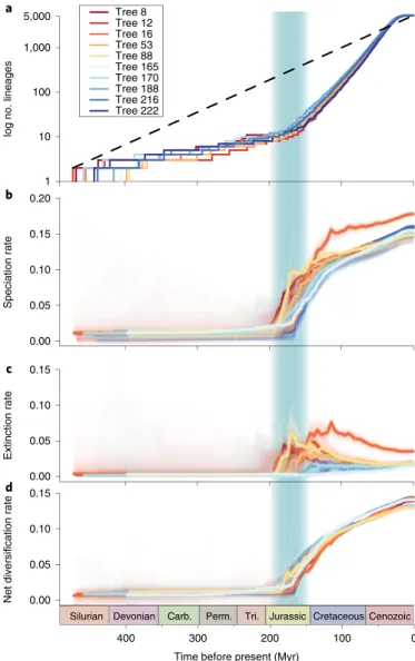
We analysed global rates of speciation and extinction in a mac- roevolutionary framework using BAMM
20. We accounted for incomplete and unequal sampling by using clade-specific sampling fractions and by ensuring that each genus was sampled in propor- tion to the number of its described species. Analyses of diversifi- cation rates in ten time-calibrated phylogenies provided evidence for rate variation through time and across lineages. Diversification rates increased abruptly at ~180 Myr ago in the early Jurassic (Fig. 2), coinciding with the breakup of Pangea, the onset of a warm, humid climate and the spread of (sub)tropical gymnosperm forests.
Consistent with this, ancestral state reconstructions suggest that the last common ancestors of most orders were likely associated with gymnosperms as hosts (Figs. 1 and 3a, Supplementary Data 3 and Supplementary Note 5), followed by multiple shifts to and diversification in association with angiosperms as hosts during the Cretaceous, similar to patterns observed in a radiation of herbivo- rous beetles
21. This agrees with observations of fungus-plant co- evolution at smaller scales
10,22, frequent host switches during fungal evolution
23and might reflect the dependence of fungi on plants as nutrient sources or mutualistic partners.
Acceleration of speciation is observed across all larger orders (Supplementary Data 4), suggestive of an external underlying cause, such as climate change or nutrient availability, instead of clade-spe- cific events. We find that the rise in speciation rates in the Jurassic is coupled with a slightly delayed increase in extinction rates ~150 Myr ago (Fig. 2). Although estimating extinction rates from phylogenies is notoriously difficult
24–26, this signal is also detected in an indepen- dent analysis using an episodic speciation/extinction model
27under a variety of conditions (Supplementary Note 6, Supplementary Fig. 6 and Supplementary Tables 3 and 4). Together, these data suggest that fungi experienced severe extinction in a period that falls close to a mass extinction event at the Jurassic/Cretaceous boundary
28, an era with a fluctuating edaphic conditions, differential extinction of several metazoan groups, and a relatively stable flora. On the other hand, we find no evidence for increased probability of extinction around the Cretaceous/Tertiary boundary, a period of severe mass extinction in plant and animal lineages. It has been hypothesized that the massive deforestation after the bolide impact has buffered fungi through the period
29, which is supported by a peak in fungal spore and hyphae fossilization right after the cataclysm
30and would explain the lack of mass extinction signal in our data.
The latitudinal diversity gradient (LDG) hypothesis posits that species richness increases from the poles towards the tropics. To test if this general prediction is valid for Agaricomycetes, we ana- lysed latitude-dependent diversification rates across all 4,429 spe- cies for which sufficient geographic data could be obtained (see Methods). Agaricomycetes display their highest species diversity and net diversification rates in the temperate zone (Supplementary Figs. 7 and 8, Supplementary Tables 5 and 6 and Supplementary Note 7), which contrasts with the diversity gradient from the poles towards the tropics in animals and plants
31. Although such a pat- tern could arise as a result of more concentrated efforts of record- ing fungi in the temperate zone, we find that the zone with highest speciation rate (between 20 and 40° in the temperate zone) does not coincide with the zone of the highest sampling density (30–60°) in our data. This suggests that our inference of a temperate peak in diversification rates is largely independent from sampling den- sity. A reversed LDG has already been implied for major fungal
0.00 0.05 0.10 0.15
Extinction rate
0.00 0.05 0.10 0.15
Time before present (Myr) 0.00
0.05 0.10 0.15 0.20
Speciation rate
Tree 8 Tree 12 Tree 16 Tree 53 Tree 88 Tree 165 Tree 170 Tree 188 Tree 216 Tree 222
1 10 100 1,000 5,000
log no. lineages
a
b
c
d
Cenozoic Silurian Devonian Carb. Perm. Tri. Jurassic Cretaceous
0 100
300 200
400
Net diversification rate
Fig. 2 | Patterns of diversification of mushroom-forming fungi through time. a–d, Lineages through time plot, a, showing the log number of lineages through time; b, speciation rate; c, extinction rate and d, net diversification rate through geologic time estimated using BAMM on ten chronograms comprising 5,284-species. 95% confidence intervals of rate estimates are shown by shaded areas. The Jurassic period is shaded in green. Carb., Carboniferous; Perm., Permian and Tri., Triassic.
groups by several surveys of environmental sequences
32–34and phylogenetic analyses
22,35, in particular for ectomycorrhizal fungi.
Although such signals might also be sensitive to biased taxonomic efforts across ecoregions, these data suggest that Agaricomycetes might not conform to broad macroecological patterns that domi- nate in animal and plant lineages.
To obtain a more resolved picture on diversification histo- ries, we analysed rate variation across clades. We identified 85 significant shifts in diversification rate (defined as shifts pres- ent in ≥50% of trees with marginal odds ratio ≥5) that included clades of diverse ages spread out across the Agaricomycetes (Fig.
1, Supplementary Data 5, Supplementary Figs. 9 and 10,Supplementary Tables 7 and 8 and Supplementary Note 8). The largest of these comprises the Agaricomycetidae, consistent with results of rate through time and lineages through time analyses, which revealed an acceleration of net diversification rates in the Jurassic (Fig. 2). Order-level shifts to higher diversification rates were inferred in the last common ancestor of the Auriculariales;
that of the Cantharellales, the Hymenochaetales (excluding the Repetobasidiaceae), the Russulales and the Agaricales (exclud- ing the hygrophoroid and pleurotoid clades (sensu Matheny
15) (Fig.
1). Most of the shifts (67%) were found in the Agaricalesand predominantly in the Paleogene, consistent with a dynamic evolutionary history of the order but also with its largest share of diversity in the class. We found accelerated diversification in the genera Coprinellus and Laccaria, as reported previously
6,7, but also in Cortinarius, Amanita and Lepiota, among others (for the complete list of shifts see Supplementary Data 5). Some of these
represent the most taxonomically diverse agaric genera, such as
Cortinarius with >2,000 (ref. 16) species described. Accelerated diversification in these groups is consistent with patterns seen in adaptive radiations
36,37. Indeed, many clades show a diversifica- tion slowdown through time, a key sign of adaptive radiations
36(Supplementary Data 6), suggesting that many of the detected shifts may feature rapid adaptive filling of available niches. Among the 85 detected shifts in diversification rates, there were several that denoted old clades with low diversity, in which the shift rep- resents a diversification slowdown rather than acceleration. For example, the genus Typhula, comprising species with minute club-shaped fruiting bodies, is an ancient group (dated at around 76 Myr) with a low diversity and an inferred diversification slow- down along its stem branch. Such parameters may indicate clades of relict lineages rooting deeply in Agaricales history but having only a few extant representatives. Taken together, these analyses provide a global view on bursts and slowdowns in the diversifica- tion history of mushroom-forming fungi and should facilitate a better understanding of adaptive diversification events in fungi, of which only a single example has been explicitly demonstrated
6.
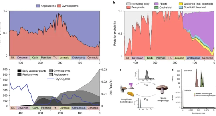
We next asked how morphological innovations may have con- tributed to shape the extant diversity of Agaricomycetes. Because fruiting body complexity is an important adaptive trait
13,14, we mapped the evolution of fruiting body morphologies on the phy- logeny and examined its impact on diversification rates. We per- formed ancestral state reconstructions and summarized inferred ancestral states through time across ten chronograms (Fig. 3b). In line with previous studies
13,14, our reconstructions suggest ancestors
0 0.03
0.02
0.01
0 600 500 400 300 200 100 700
0 0.5 1.0
Species diversity O2/CO2 rati
o
Pteridophytes Angiosperms Gymnosperms Early vascular plants
No fruiting body
Cyphelloid
Gasteroid (incl. secotioid) Pileate
Coralloid/clavarioid Resupinate
O2/CO2 ratio
Non-pileate morphologies
Pileate morphology q01
q10
0 1 2 3
Density
0.5
0 1.0 1.5
0 5 10
Density
0.5
0 1.0 1.5
b a
c d
0 50 100 150 200 Speciation
Density
0 5,000 10,000 15,000 Extinction
Density
0 0.025 0.05 0.075 0.1
Evolutionary rate Non-pileate morphologies Pileate morphologies
Angiosperms Gymnosperms
0 0.5 1.0
Posterior probability Posterior probability
Cenozoic Sil. Devonian Carb. Permian Tri. Jurassic Cretaceous
0 100
300 200
400
Cenozoic Sil. Devonian Carb. Permian Tri. Jurassic Cretaceous
0 100
300 200
400 Cenozoic
Sil. Devonian Carb. Permian Tri. Jurassic Cretaceous
0 100
300 200
400
Fig. 3 | The evolution of morphological and nutritional traits of mushrooms through time. a, The evolution of substrate association through geologic time (top) and the evolution of vascular plant diversity and O2/CO2 levels (bottom, adapted from Niklas41 and Berner42. Inferred ancestral probabilities of fruiting body types were summarized across the ten phylogenies, by splitting the time scale of each tree into 100 bins and summing probabilities across the tree. b, The evolution of fruiting body types through time and the radiation of the agaricoid morphology since the Jurassic. Plot created as in a. For details of character coding and ancestral state reconstructions and detailed results, see Supplementary Note 5. c, Schematic model of the evolution of pileate-stipitate morphologies. The posterior distribution of transition rates from non-pileate (left) towards pileate-stipitate forms (right) and vice versa are shown above the arrows. Rates were estimated by Markov chain Monte Carlo (MCMC) in BayesTraits. d, Posterior distribution of trait-dependent speciation and extinction rates estimated under the binary state speciation and extinction (BiSSE) model for non-pileate versus pileate-stipitate fruiting body morphologies. Carb., Carboniferous; Perm., Permian and Tri., Triassic.
NATURE ECOLOGy & EVOLUTION | VOL 3 | APRIL 2019 | 668–678 | www.nature.com/natecolevol
with resupinate (crust-like) fruiting bodies for most early nodes along the backbone of the Agaricomycetes. The early dominance of resupinate morphologies was rapidly taken over by an array of more complex morphologies in the late Jurassic (~170–180 Myr), of which the pileate-stipitate type appears most dominant. This pat- tern could have been driven by the radiation of Agaricomycetidae, which contains the majority of pileate-stipitate species and started to diversify around this period, although pileate-stipitate species evolved in 12 orders as well, including the Russulales, Cantharellales and Gloeophyllales, among others. In the meanwhile, resupinate lineages may have simply continued to diversify at their previous rate, but, because of the radiation of species with pileate-stipitate fruiting bodies their dominance was diminished at the scale of the entire class. Consistent with this view, gains of the pileate-stipitate morphology are estimated to be significantly more likely (7–50 times, log(Bayes factor), logBF
= 47) than their loss, indicating atrend towards pileate-stipitate morphologies, as reported earlier
13. In fact, the pileate-stipitate morphology evolved convergently in at least 33 clades, suggesting it represents a stable attractor in the mor- phospace. Nevertheless, the probability of the loss of pileate-stip- itate morphology is significantly larger than zero (logBF
= 157.2),reflecting evolutionary transformations of pileate-stipitate fruiting bodies happening in many groups (Fig. 3c and Supplementary Data 1 and 7). We tested the impact of fruiting body morphologies on diversification rate in a character-state-dependent speciation and extinction framework
38,39. Clades with pileate-stipitate fruiting bod- ies have a significantly higher speciation rate (P < 10
−16, likelihood ratio test, LRT) than clades with other morphologies (Fig. 3d and Supplementary Data 7). This may be because the pileate-stipitate morphology provides support and protection for developing spores (for example, from precipitation) and enhances their dispersal efficiency by raising sporogenous tissue above ground-level; these advantages may explain how pileate-stipitate fruiting bodies can promote diversification and suggest they represent a key innovation for mushroom-forming fungi
Conclusions
This study represents a global analysis of the dynamic evolu- tionary history of mushroom-forming fungi. The diversity of Agaricomycetes might have been shaped by both class-wide diversi- fication rate shifts and explosive clade-specific events. We identified a major class-wide radiation of Agaricomycetes in the Jurassic, which possibly followed a warming and humid climate in this period. The onset of this radiation coincided with the expansion of angiosperms and followed patterns of gymno- and later angiosperm expansion during the Mesozoic-Cenozoic radiation
40. Our analyses provide evidence for several clade-specific adaptive radiations in the class, offering a possible explanation for why some genera contain a sin- gle species, while others contain thousands. Our data display strong signal for a mass extinction event coinciding with increased extinc- tion rates at the Jurassic/Cretaceous boundary, however, no such evidence was found in the Agaricomycetes for the much more influ- ential Cretaceous–Tertiary mass extinction event. The evolution of pileate-stipitate fruiting bodies, that is, morphologies with cap and stipe might be a key driver of evolutionary radiations, suggesting that the convergent evolution of the classic mushroom morphology contributed to shaping extant diversity in the Agaricomycetes. We predict that further data on traits and ecological opportunities that generated the spectacular diversity of mushroom-forming fungi will help to elucidate the general principles of mushroom evolution and integrate this ecologically important group into the record of major biodiversification events.
Methods
Molecular biology methods. Genomic DNA was extracted from 0.1–10 mg of dried herbarium specimens using the DNeasy Plant Mini kit (Qiagen) or the
Nucleospin Plant II mini kit (Macherey-Nagel) following the manufacturers’
instructions. PCR amplification was performed as described previously6,15 on the LSU of the nuclear ribosomal RNA with the LR7 and LROR primers. Sequencing was performed commercially using the same primers as used for PCR. Sanger reads were assembled to a contig using the Pregap and Gap4 programs of the Staden package43 and checked manually against the electropherograms.
Taxon sampling. We sampled herbarium specimens so that taxon sampling be proportional across clades and geographic regions. To that end, we initially obtained estimates of the known diversity for each of the genera from Species Fungorum44 (http://www.speciesfungorum.org), the Dictionary of the Fungi16 and Funga Nordica45. Taxonomic information from these sources was compiled for all genera of Agaricomycetes. Using this compilation, we calculated the number of target species that needed to be sampled for each genus to obtain a final dataset of
~5,000 species (~30% sampling of total diversity) in which sampling of species in each genus is proportional to their described diversity. Although the three sources differed in their completeness, geographic scope (Dictionary of the Fungi and Species Fungorum being global databases and Funga Nordica being, taxonomically, the most stringent of the three) and taxonomic concept, it gave us general guidance on how to keep taxon sampling proportional across genera. When sampling species within genera, attempts have been made to obtain specimens from undersampled geographic regions—in particular, Africa, Asia, Australasia and South America.
Sequence alignment. Multiple sequence alignment was carried out for the LSU, ef-1a and RPB2 loci separately using the Probabilistic Alignment Kit (PRANK release 140603)46,47. An iterative alignment refinement strategy as described in Tóth et al.48 was employed: maximum-likelihood gene trees computed from preliminary alignments (using RAxML, see below) were used as guide trees for the next round of multiple alignment for PRANK. After three rounds of iterative refinement, the alignments were further corrected manually using a text editor.
Manual curation was restricted to correcting homologous regions erroneously juxtaposed by PRANK. Alignments of individual sequences were concatenated into a superalignment. The concatenated alignment is available at Dryad (accession number doi:10.5061/dryad.gc2k9r), GenBank accession numbers for all sequences used are shown in Supplementary Data 1.
Genome and transcriptome sequencing and assembly. Sequencing. The genomes of Coprinopsis marcescibilis, Crucibulum laeve, Dendrothele bispora, Heliocybe sulcata, Peniophora sp., Pluteus cervinus, Polyporus arcularius and Pterula gracilis were sequenced using a combination of fragment and long-mate pair Illumina libraries. In addition, the genome of Coprinellus micaceus was sequenced using Pacific Biosciences platform. Fragment Illumina genomic libraries were produced for 100 ng of DNA was sheared to 270 bp using the Covaris LE220 and size selected using SPRI beads (Beckman Coulter). The fragments were treated with end repair, A-tailing and ligation of Illumina compatible adaptors (IDT, Inc.) using the KAPA- Illumina library creation kit (KAPA biosystems). For long-mate pair libraries (C. laeve, D. bispora, H. sulcata, P. arcularius and P. gracilis), 5 μg of DNA was sheared using the Covaris g-TUBE and gel size selected for 4 kb. The sheared DNA was treated with end repair and ligated with biotinylated adaptors containing loxP.
The adaptor ligated DNA fragments were circularized via recombination by a Cre excision reaction (NEB). The circularized DNA templates were then randomly sheared using the Covaris LE220 (Covaris). The sheared fragments were treated with end repair and A-tailing using the KAPA-Illumina library creation kit (KAPA Biosystems) followed by immobilization of mate pair fragments on strepavidin beads (Invitrogen). Illumina compatible adaptors (IDT, Inc.) were ligated to the mate pair fragments and eight cycles—or in the case of Heliocybe sulcata ten cycles—of PCR were used to enrich for the final library (KAPA Biosystems). For C. micaceus unamplified libraries were generated using the Pacific Biosciences standard template preparation protocol. Then, 5 μg of genomic DNA was used to generate each library and the DNA was sheared using Covaris g-Tubes to generate sheared fragments of 10 kb in length. The sheared DNA fragments were then prepared using the Pacific Biosciences SMRTbell template preparation kit, where the fragments were treated with DNA damage repair, had their ends repaired so that they were blunt-ended and 5’ phosphorylated. Pacific Biosciences hairpin adaptors were then ligated to the fragments to create the SMRTbell template for sequencing. The SMRTbell templates were then purified using exonuclease treatments and size selected using AMPure PB beads.
All transcriptomes in this study were sequenced using Illumina RNA-Seq.
Stranded complementary DNA libraries were generated using the Illumina Truseq Stranded RNA LT kit. Messenger RNA was purified from 1 μg of total RNA using magnetic beads containing poly-T oligos. mRNA was fragmented and reversed transcribed using random hexamers and SSII (Invitrogen) followed by second strand synthesis. The fragmented complementary DNA was treated with end-pair, A-tailing, adaptor ligation and ten cycles or, in the case of C. marcescibilis, C. laeve and P. cervinus, eight cycles of PCR.
The prepared Illumina libraries were quantified using KAPA Biosystem’s next-generation sequencing library quantitative PCR kit and run on a Roche LightCycler 480 real-time PCR instrument. The quantified libraries were then multiplexed with other libraries, and the pool of libraries was then prepared for
sequencing on the Illumina HiSeq sequencing platform using a TruSeq paired-end cluster kit, v.4 and Illumina’s cBot instrument to generate a clustered flow cell for sequencing. Sequencing of the flow cell was performed on the Illumina HiSeq2500 sequencer using HiSeq TruSeq SBS sequencing kits, v.4, following a 2 × 150 indexed run recipe. In the case of C. micaceus, Dendrothele bispora, Peniophora sp. and P.
arcularius, TruSeq paired-end cluster kit, v.3, and TruSeq SBS sequencing kits, v.3, were used and in the cases of C. laeve, H. sulcata and P. gracilis a 2 × 100 indexed run recipe was performed.
For PacBio sequencing primer was annealed to the SMRTbell templates and Version P5 sequencing polymerase was bound to them. The prepared SMRTbell template libraries were then sequenced on a Pacific Biosciences RSII sequencer using Version C3 chemistry and 1 × 240 min sequencing movie run times.
Assembly and annotation. Genomic reads from each pair of Illumina libraries were QC filtered for artefact/process contamination and assembled together with AllPathsLG v.R4940349. Illumina reads of stranded RNA-seq data were used as input for de novo assembly of RNA contigs and assembled into consensus sequences using Rnnotator (v.3.4)50. The Pacific Biosciences sequence data were filtered with smrtanalysis assembled together with Falcon version 2014082 (ref. 51), improved with finisherSC52 and polished with Quiver. All genomes were annotated using the JGI Annotation Pipeline and made available via the JGI fungal portal MycoCosm53. Genome assemblies and annotation were also deposited at DDBJ/
EMBL/GenBank.
Phylogenomic analysis of 104 Agaricomycotina. Phylogenomic analysis.
The genome sequences of 104 species (Supplementary Table 1) were included in the phylogenomic analysis of Agaricomycotina. Two representatives of Tremellomycetes (Tremella mesenterica (Treme1), Cryptococcus neoformans var.
grubii H99 (Cryne_H99_1)) were used as outgroups.
We performed all-versus-all blast using mpiBLAST 1.6.0 (ref. 54) with default parameters, then identified gene families using the Markov clustering algorithm MCL 14-137 (ref. 55) with an inflation parameter of 2.0. We first identified gene families that contained 52–208 genes (50–200% of the species included in the study), then performed multiple sequence alignment using PRANK 140603(ref. 47).
Ambiguously aligned regions were removed from the alignments using Gblocks 091b56 with the settings -p = yes -b2 = 26 -b3 = 10 -b4 = 5 -b5 = h -t = p -e = .gbl.
Next, we screened for gene families that contained a single representative gene for each species, or ones that contained inparalogs but no deep paralogs. Deep paralogs were identified following Nagy et al.57. Gene trees were inferred using the PTHREADS version of RAxML 8.1.2 (ref. 58) using the PROTGAMMAWAG model and the standard algorithm. A single inparalog, closest to the root on the basis of root-to-tip patristic distances was retained for each species. Gene families in which 75% or more of the species were represented were concatenated into a supermatrix.
We used RAxML 8.1.2 to perform maximum-likelihood analysis and bootstrapping on the concatenated dataset, under a WAG model with gamma- distributed rate heterogeneity partitioned by gene. We ran 100 bootstrap replicates using the rapid hill-climbing algorithm. Because in initial analyses Peniophora sp., Tubaria furfuracea and Clavaria fumosa were placed on long terminal branches, we performed the following steps to clean the alignments of overly divergent sequences (either due to sequencing errors or pseudogenes). We screened all individual gene trees and excluded proteins with a terminal branch length >2.75 times longer than the average branch length of the gene tree. Altogether, 1,294 (in 542 gene families) protein sequences were excluded from the analyses.
Sensitivity analysis. The robustness of the dataset was tested by eliminating incrementally higher numbers of fast-evolving sites using six levels of stringency in Gblocks 091b56. Using these parameters, we eliminated 8.5% (-b1 = 78 -b2 = 78 -b3 = 10 -b4 = 10), 24.3% (-b1 = 78 -b2 = 78 -b3 = 8 -b4 = 15), 36.7% (-b1 = 88 -b2 = 88 -b3 = 8 -b4 = 15), 46.4% (-b1 = 95 -b2 = 95 -b3 = 8 -b4 = 15), 50.1%
(-b1 = 100 -b2 = 100 -b3 = 8 -b4 = 15) and 55.2% (-b2 = 104 -b3 = 5 -b4 = 20) of the least reliably aligned regions of the alignments, resulting in trimmed concatenated datasets with 129,886, 107,496, 89,732, 76,153, 70,862 and 63,309 amino acid sites, respectively. We performed maximum-likelihood phylogenetic inference for each of the reduced datasets in RAxML as described above.
Maximum likelihood analyses of the 5,284-taxon dataset. Maximum-likelihood trees for the 5,284-taxon dataset were inferred using the parallel version of RAxML v.8.1.2 (ref. 58) under the generalized time-reversible model with gamma- distributed rate heterogeneity (four categories) with three partitions corresponding to the LSU, ef1-α and rpb2 loci. The phylogenomic tree was used as a backbone monophyly constraint. We performed 245 maximum-likelihood inferences and tested whether these trees adequately represented the plausible set of topologies given the alignment. This was done to ensure that phylogenetic uncertainty is properly taken into account in subsequent comparative analyses. If our tree set contains all plausible topologies, then the rolling average of pairwise Robinson–
Foulds distances should show a saturation as a function of increasing the number of trees. To this end, we computed Robinson–Foulds distance for each pair of trees for incrementally larger numbers of trees using R package ‘phangorn’ v.2.0.2 (ref. 59). We then plotted the rolling average, maximum and minimum values as a function of the number of trees in R.
Molecular clock dating of the 5,284-taxon dataset. Due to computational limitations, we focused on ten maximum-likelihood trees that maximize topological diversity (as inferred on the basis of Robinson–Foulds distances) as representative trees for molecular clock analysis. These were chosen by first calculating pairwise Robinson–Foulds distances between trees, then hierarchically clustering trees using Ward’s clustering method (as implemented in the hclust R function). The ten maximum-likelihood trees for subsequent analyses were chosen evenly from the resulting clusters of trees. To overcome the computational limitations of inferring accurate chronograms for thousand-tip phylogenies, we adopted a two-step strategy. First, PhyloBayes 4.1b60 was used to infer parameters of a birth-death model and divergence times of trees on 10% subsampled versions of the 5,284-taxon dataset. Subsampled datasets were obtained by randomly deleting 90% of the species, but forcing key descendants of fossil-calibrated nodes to be retained in the subsampled alignments. Then we used the ages and parameters estimated in PhyloBayes as input parameters for FastDate development version61 (provided by T. Flouri) for analysing the complete 5,284-species dataset.
PhyloBayes analyses were run using the 10% subsampled dataset, a birth-death prior on divergence times, an uncorrelated gamma multiplier relaxed clock model and a CAT-poisson substitution model with a gamma distribution on the rate across sites. A uniformly distributed prior was applied to fossil calibration times.
All analyses were run until convergence, typically 15,000 cycles. Convergence of chains was assessed by visually inspecting the likelihood values of the trees and the tree height parameter. We sampled every tree from the posterior and after discarding the first 7,000 samples as burn-in we summarized the posterior estimates using the readdiv function of PhyloBayes.
Next, we used FastDate, a program that implements the speed dating algorithm described in Akerborg et al.61. FastDate was run on the complete trees (5,284 species) with the node ages constrained to the values of the 95% highest posterior densities of the ages inferred by PhyloBayes. FastDate analyses were run with time discretized into 1,000 intervals and the ratio of sampled extant individuals set to 0.14.
Fossil calibrations. The extensive sampling density of our tree allowed us to use more fossil calibration points than any study before and to place them more precisely within the tree. Eight fossils were used as calibration points (Supplementary Table 2) for the crown node of the specified taxa.
We excluded a number of prospective well-preserved fossils for reasons of redundantly calibrating an already calibrated node (Appianoporites vancouverensis—Hymenochaetales62, Protomycena electra—marasmioid clade63, Cyathus dominicanus—Nidulariaceae64, Fomes idahoensis—Polyporales65. Geastrum tepexensis66 was not considered as it could be assigned to either of the two earth- star clades, one in the Phallomycetidae (Geastraceae) or the other in the Boletales (Astraeus). For other mushroom fossils, the taxonomic affiliations were deemed too uncertain.
To investigate if there is any conflict between the fossil calibration points we conducted a fossil cross-validation analysis following Near et al.67. For this, we ran PhyloBayes analyses on one of the 10% subsampled trees with the same settings as mentioned above, using a single fossil calibration point at a time. This resulted in eight independent molecular dating analyses. To quantify conflict between single fossil calibrations, first we calculated the sum of the square differences between molecular age estimates and fossil ages:
∑
=
≠
D SSx
i x i2
where x is the fossil calibration point used and Di is the difference between molecular age estimate and fossil age for fossil i. We ordered the SS values of each of the eight analyses in descending order and calculated the average squared deviation for all fossil calibrations:
=∑ ∑
−
= ≠
s D
n n( 1)
nx i x i
1 2
Next, the analysis with the highest SS value was removed and s was recalculated. We continued this process until only two analyses remained. In parallel, we performed one-tailed F-tests to check whether the removal of the fossil had a significant effect on the variance of s. The principle of this procedure is that during the stepwise removal of fossils, s should decrease by small constant values and variance should not decrease significantly
Genome-based molecular clock analyses. We examined the robustness of our molecular age estimates using phylogenomic methods as an alternative to the 5,284 species phylogeny. Specifically, we tested whether the differences between our and previous17,18 molecular clock estimates for Agaricomycete orders were attributable to differences in the dataset or analytical method used or a difference in how precisely fossils could be placed on the tree. To this end, we performed a series of molecular clock analyses on our phylogenomic dataset that resembled that of Kohler and Floudas in terms of topology and taxon sampling density, but differed in the placement of some fossil calibrations. A key difference was that our phylogenomic tree included the most recent common ancestor (MRCA) of the Hymenochaetales and that of the Suillaceae, which allowed us to calibrate the MRCA of these clades, NATURE ECOLOGy & EVOLUTION | VOL 3 | APRIL 2019 | 668–678 | www.nature.com/natecolevol
as opposed to their stem nodes by Kohler et al.18 and Floudas et al.17 Further, our analysis includes the MRCA of the Nidulariaceae, a relatively recent node that can be calibrated by two well-preserved fossils described recently64
Phylogenomic dataset. We used a smaller, more conserved subset of the 568-gene and 104-species phylogenomic dataset (which was computationally not tractable in these analyses). First, we selected the first 70 most conserved genes of the 568-gene dataset by calculating the mean genetic distances for each gene using the dist.alignment function of the seqinR R package v.3.4-5 (ref. 68). To enable a more accurate placement of fossil calibration points we added additional three species (Cyathus striatus, Pycnoporus cinnabarinus, Suillus brevipes) to this dataset (Supplementary Table 1) and excluded two taxa that harboured ambiguous positions. We searched homologous sequences in the additional genomes using blastp v.2.7.1 (ref. 69) with one randomly selected gene from each of the 70 gene families as query. We selected the best hit (smallest E-value) as a one-to-one ortholog if the second best hit had a significantly worse E-value (by 20 orders of magnitude). Protein clusters were aligned by PRANK v.100802 (refs. 46,47) using default settings. Next, conserved blocks of the alignments were selected using Gblocks v.0.91b56 with default settings except for the minimum length of a block that was set to 5 and gap positions in half of the sequences were allowed. A phylogenomic tree was constructed by RAxML v.8.2.11 (ref. 58) under the WAG + G substitution model partitioned by gene.
Calibrations. To dissect sources of differences in molecular age estimates, we ran analyses under three fossil calibration schemes (Supplementary Data 2) and the 105-species phylogenomic tree. First, we used the same fossil calibration scheme as for the 5,284-species phylogenetic dataset (‘Default calibration scheme’).
Next, we replicated the analyses of Kohler et al.18 on our tree, using the fossil calibration points from Kohler et al. (‘Kohler et al. calibration scheme 1’). For this, we placed the suilloid ectomycorrhiza fossil in the split of Suillinae/Paxillinae/
Sclerodermatinae and Archaeomarasmius leggettii in the MRCA of Gymnopus luxurians and Schizophyllum commune with uniformly distributed 40–60 Myr and 70–110 Myr ago time priors, respectively. Finally, we used the calibrations used by Kohler et al. (scheme 2) but placed the two fossils in the MRCAs of the Suillaceae and marasmioid clade, respectively (Kohler et al.18 calibration scheme 2’). In all analyses we constrained the age of the root to be between 300 Myr and 600 Myr ago.
Penalized likelihood analysis in r8s. We ran a series of molecular clock analyses in r8s v.1.81 (ref. 70). A cross-validation analysis was performed to determine the optimal smoothing parameter (λ) by testing values across seven orders of magnitude starting from 10−3. The additive penalty function was applied and the optimization was run 25 times starting from independent starting points. In one optimization step, after reaching an initial solution, the solution was perturbed and the truncated Newton optimization was rerun 20 times. We compared the results of previous studies to that of analyses across seven ancestral nodes in Agaricomycotina (Supplementary Data 2).
Bayesian molecular clock dating. We used the mcmctree method implemented in PAML v.4.8a71. The independent-rates clock model, a WAG substitution model and approximate likelihood calculation72 were used. The birth rate, the death rate and the sampling fraction of the birth-death process were set to 1, 1 and 0.14, respectively.
The shape and the concentration parameter of the gamma-Dirichlet prior for the drift rate coefficient (σ2) was set to 1 and three different scale parameters were tested (10, 100, 1,000) to see their effect on the time estimates. The substitution rates of each gene were estimated by codeml under a global clock model, to set the parameters of the gamma-Dirichlet prior for the overall rate. By calculating the mean substitution rate of the loci and examining the density plot of the rates we set up a prior that reasonably fitted the data: the shape parameter, the scale parameter and the concentration parameter were set to 5, 90.7441 and 1, respectively, resulting in an average substitution rate per site per time unit of 0.055. We set the time unit to 100 Myr and applied uniform priors on eight fossil calibrations with lower and upper hard bounds. MCMC analysis was run for 80,000 iterations, discarding the first 20,000 iterations as a burn-in and sampling every 30th tree from the posterior. After three independent analyses were run the convergence of log-likelihood values was visually inspected and the estimated ages were compared between replicates.
Analyses of diversification and character evolution. Character coding. We discretely coded three characters, the presence of a cap, fruiting body type and substrate preference for the 5,284 species. Fruiting body types were coded as one of six types and data were compiled from the literature. The six character states distinguished were: (0) no fruiting body; (1) resupinate; (2) agaricoid;
(3) cyphelloid; (4) gasteroid/secotioid and (5) coralloid/clavarioid. Transitional morphologies, or species for which no clear decision could be made on fruiting body type were coded as uncertain. Resupinate fruiting bodies were defined as crust-like or effused, flat morphologies that follow the morphology of the substrate, but irrespective of thickness or hymenophore type. The agaricoid type was defined as having a distinguishable stipe and cap. Cyphelloid species were coded following Bodensteiner73. The gasteroid types included species with closed fruiting bodies that produce spores internally. No distinction was made between secotioid,
sequestrate and false-truffle morphologies and all were coded as gasteroid. Fruiting bodies with club-shaped or branched, erect morphology but no differentiated cap were considered coralloid/clavarioid.
The presence of a cap, that is pileate-stipitate morphology, was coded on the basis of literature data as either absent (state 0) or present (state 1). Species with rudimentary or reduced caps were coded as uncertain.
We coded species’ preference for substrate on the basis of literature data (a detailed listing of resources used is not given) as gymnosperm, angiosperm or both (that is, generalist species). Species were considered gymno- or angiosperm specialists if >90% of records were for either plant group, or their habitat preferences in taxonomic literature were described by the terms
‘exclusively’, ‘predominantly’, ‘mostly’ or occurring on the least dominant substrate ‘rarely’, ‘very rarely’ or ‘exceptionally’. On the other hand, species having records on both gymno- and angiosperm substrates, described in the literature as generalists or given multiple gymno- or angiosperm substrate plant species were coded as generalists. Species with insufficient data or no data at all were treated as missing data. Soil-inhabiting saprotrophs were coded on the basis of their association with either gymno- or angiosperms, if a clear preference was reported in the literature.
Tests of the LDG hypothesis. Global positioning system (GPS) data. We downloaded 5,884,445 fungal GPS records from the GBIF database, representing 4,429 Agaricomycetidae species. For 848 species, a location based on the province, country and/or biogeographic realm74 was obtained from the literature. In cases where only the province, country or biogeographic realm was available, we took the centroid of the area as a proxy for GPS location. All GPS data were handled and processed in R75. Noise was added to identical GPS coordinates using the jitter function in R.
Analyses of geographic diversification. State-dependent diversification rates were estimated in two ways: (1) using centroid latitudes as continuous traits (for example, Sánchez-Ramírez et al.35) and (2) using discrete areas. We used the data mentioned above to first calculate a centroid coordinate (RGEOS R package) in cases where multiple GPS records exist per species. Then we took the centroid latitude for each species. For singletons, we simply took the latitude of each record.
We also used the GPS database to calculate a standard deviation for latitude per species. For species with a single record, we took the mean standard deviation of species with multiple records. We fitted multiple Quantitative State Speciation and Extinction (QuaSSE76) models, using a maximum-likelihood approach, to ten of the 5,284-species chronograms. Models included speciation rate changes as a constant function of the trait (no effect), as a linear function or as a Gaussian function, keeping the extinction rate constant76. We also added two models in which the extinction rate varied as linear or Gaussian functions, while speciation rate remained constant. To improve the efficiency of the algorithm given the scale of the tree, we applied the following settings to the models: method = ’fftC’, dt.max = 1 and nx = 256. Akaike information criterion values were averaged across phylogenies and compared between different models. We used the best supported model to interpolate speciation rates into a 1 × 1 degree global map made with Natural Earth. (Free vector and raster map data are available at www.
naturalearthdata.com.)
To obtain discrete areas, first we divided all terrestrial WWF ecoregions into either tropical or extra-tropical. For tropical areas we considered: Tropical and Subtropical Moist Broadleaf Forests, Tropical and Subtropical Dry Broadleaf Forests, Tropical and Subtropical Grasslands, Savannas and Shrublands. All other terrestrial ecoregions were deemed extra-tropical. Ecoregion polygons were integrated (that is, dissolved) in a way that only two-state areas were found (Supplementary Note 7). For species with multiple GPS records, we extracted binary information about their presence in both areas. For records that were not found precisely within the geometry of the area, we took the area to which the distance to the GPS point was closer. To assign discrete states to each species with multiple records, our criterion was to assign a ‘widespread’ state (both areas) if records for the area with the minor frequency was higher than 0.2. In any other case, we assigned ‘tropical’ or ‘extra-tropical’ states to taxa in the area with the highest frequency. For taxa that had only biogeographic realm data, we coded them as follows: ‘widespread’: Neotropical, Afrotropical, Oceanian/Australia; ‘tropical’:
Panamenian, Oriental and extra-tropical': Europe/Palaearctic/North Asia, Nearctic, Saharo-Arabian, Sino-Japanese. Using these three states for each taxon, we fitted multiple constrained models and one full model of Geographic State Speciation and Extinction (GeoSSE77) in a maximum-likelihood framework. The full model consisted of seven parameters: (1) speciation rate in the tropics, (2) speciation rate in the extra-tropical zone, (3) the allopatric speciation rate (speciation rate in both tropical and extra-tropical regions), (4) extinction rate in the tropics, (5) extinction rate in the extra-tropical zone, and dispersal rates to (6) the tropics and to (7) the extra-tropical zone. The constrained models consisted of: (1) speciation in the tropics is equal to speciation in the extra-tropical zone; (2) extinction in the tropics is equal to extinction in the extra-tropical zone and (3) dispersal to the tropics occurs at the same rate as dispersal to the extra-tropical zone. In each case, a single parameter for speciation, extinction, and dispersal was respectively estimated, allowing the other parameters of the model to vary. To explore the parameter space