(will be inserted by the editor)
Global dynamics of an epidemiological model with age-of-infection dependent treatment rate
Gergely R¨ost · Toshikazu Kuniya · Seyed M. Moghadas · Jianhong Wu
Received: date / Accepted: date
Abstract We revisit a previously established model for influenza transmis- sion dynamics, in which antiviral treatment as a single containment strategy was administered within a specified window of opportunity for initiating treat- ment. We extend this model to a more general framework with age-of-infection dependent treatment rates. The resulting age structured model can be trans- formed into a closed system of delay differential equations, for which we per- form a complete global stability analysis. By constructing suitable Lyapunov functions, we show that the effective reproduction number fully characterizes the possible outcomes of disease dynamics. Our results allow us to evaluate treatment strategies and examine the impact of treatment delays on the po- tential success of disease control.
Keywords age of infection · epidemiological model · delay · Lyapunov function·disease control
1 Introduction
The classical SIR (Susceptible-Infected-Recovered) model of disease transmis- sion [10] provides a basic framework for most compartmental epidemic models.
The degree of complexity in such models is largely determined by the immuno- logical and epidemiological characteristics of the disease. One example that im-
Gergely R¨ost
Bolyai Institue, University of Szeged, Hungary E-mail: rost@math.u-szeged.hu
Toshikazu Kuniya
Graduate School of System Informatics, Kobe University, Japan Seyed M. Moghadas
Agent-Based-Modelling Laboratory, York University, Toronto, Canada M3J 1P3 Jianhong Wu
Department of Mathematics and Statistics, York University, Toronto, Canada M3J 1P3
mediately comes to mind is influenza, which is a respiratory infection mainly caused through human-to-human transmission of small particle aerosols. The dynamics of influenza spread, and many other infectious diseases with similar characteristics, in a population can be described by a model that comprises the classes of susceptible, exposed (infected but not infectious), asymptomatic (in- fectious without developing clinical symptoms), pre-symptomatic (infectious before the symptoms appear), and symptomatic (infectious with clinical symp- toms) individuals. However, this structure may even become more complex when applying the model to evaluate the effectiveness of intervention strate- gies, such as treatment of symptomatic infection. It has been shown that an effective course of influenza therapy requires the prompt onset of treatment within 48 hours of the onset of clinical symptoms [16]. In practice, however, diagnosis of most infected cases and therefore start of treatment is associated with a delay after the symptoms appear. In a previous study [1], we have shown that such delay can be incorporated into the model as an independent structure variable, by monitoring the density of infected individuals in terms of the time elapsed since the onset of clinical disease. The model, formulated as a system of delay differential equations, enabled us to determine the condi- tions for disease eradication in terms of the population-level of treatment and delay in start of treatment.
While treatment remains a key component of infection management strate- gies for several diseases, the timing for initiation of treatment can have a sig- nificant impact on the short- and long-term disease epidemiology in the pop- ulation [2, 15, 9]. This is particularly relevant to the development and spread of drug-resistance, which remain an important global public health concern.
For example, recent studies show that, depending on the probability of re- sistance development at the host level and the relative transmission fitness of the resistant-type at the population level, the minimum infection state of the system at equilibrium for competing pathogen subtypes may occur with considerable delay in start of the treatment during the infectious period [9].
Although such delay in start of treatment could play a critical role in dis- ease dynamics, current treatment practices largely pivot towards management of infection and severe outcomes in patients, leaving out the possible evolu- tion and epidemiological consequences of resistance spread under the selection pressure of drugs. The impact of delay as a control parameter has also been recognized in vaccine-preventable diseases for scheduling booster doses in order to determine the optimal timing of vaccination for generating a longer term herd protection and reducing the impact of disease on the population [18].
Collectively, these studies suggest that the ‘delay’ term in epidemic models could reveal important factors that influence disease dynamics, and pertinent strategies for control and prevention.
In this paper, we revisit the work of Alexander et al. [1] and extend the model to include demographic turnover and study the conditions for disease propagation in the population in the context of age-of-infection dependent treatment rates and delay in start of treatment. We identify the effective re- production number and show that when it is less than unity [1], the disease
will be eradicated from the population. On the other hand, when the repro- duction number of disease transmission exceeds the unity, by constructing a Lyapunov function we prove the global stability of a unique endemic equilib- rium. Therefore, the effectiveness of the treatment strategy for disease control is fully characterized by the reproduction number as a threshold parameter.
In what follows, we provide the structure of the model and its analysis, which relies on the general framework developed in our previous work [1].
2 The model
Our starting point is the model of Alexanderet al.[1], and we extend that to include a constant recruitment rate (Λ) into the susceptible population, and a natural death rate (γ). The population is divided into the compartments of susceptible, exposed (infected but not infectious), asymptomatic and symp- tomatic infected individuals. Denoting susceptible and exposed classes by S andE, assuming mass action incidence we have
S0(t) =Λ−βS(t)Q(t)−γS(t) (1) and
E0(t) =βS(t)Q(t)−µEE(t)−γE(t), (2) where β is the baseline transmission rate, 1/µE represents the lentgh of in- cubation period, and Q(t) is the force of infection, to be formulated below.
Let p∈ [0,1] be the probability for an exposed individual to develop symp- toms. Asymptomatic individuals (A) may possibly shed pathogen during their infectious period (1/µA), and this compartment follows
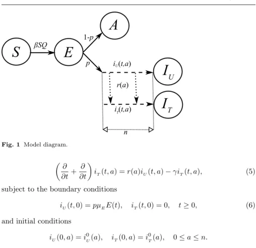
A0(t) = (1−p)µEE(t)−µAA(t)−γA(t). (3) Only symptomatic infected individuals may receive treatment within a window of opportunity for efficient treatment, and to accurately track the treated and untreated symptomatic infection, we structure this class with respect to the time elapsed since the start of infection, denoting the density of untreated and treated infected individuals with respect to age-since-infectionaat timetby iU(t, a) andiT(t, a), respectively. We divide the infectious period of the symp- tomatic infection into two stages. The primary stage represents the window of opportunity for initiating therapy, and it terminates at time since infection a=n. We assume that individuals do not recover during this primary stage, neither die due to the disease. Individuals who have initiated treatment during this window will progress to the secondary stage and receive no treatment for the entire course of symptomatic infection.
Now we consider the equations governing the disease dynamics within the primary stage. Assuming that the treatment rate at time aafter the onset of symptoms isr(a), we have fora∈[0, n] that
∂
∂t+ ∂
∂t
iU(t, a) =−r(a)iU(t, a)−γiU(t, a), (4)
S E
A
I I
iU (t,a)
i (t,a)
r(a) U
T p
βSQ 1-p
T
n
Fig. 1 Model diagram.
∂
∂t+ ∂
∂t
iT(t, a) =r(a)iU(t, a)−γiT(t, a), (5) subject to the boundary conditions
iU(t,0) =pµEE(t), iT(t,0) = 0, t≥0, (6) and initial conditions
iU(0, a) =i0U(a), iT(0, a) =i0T(a), 0≤a≤n.
Let IU(t) and IT(t) denote, respectively, the total number of untreated and treated infected individuals in the secondary stage, whena≥n. Their dynam- ics is governed by
I0
U(t) =iU(t, n)−(µU +dU)IU(t), I0
T(t) =iT(t, n)−(µT +dT)IT(t), (7) where 1/µU and 1/µT are the mean secondary infectious periods, and dU and dU represent disease induced mortality rates of untreated and treated individuals, respectively. See Figure 1 for the flowchart of the dynamics.
Next we formulate the last remaining component of the model, the force of infectionQ(t). To this end, we introduce the parametersδA,δU, representing transmissibility during asymptomatic and secondary stage infection, relative to the primary stage symptomatic infection; andδT denotes the reduction of transmission due to therapy. This way, using mass action, we obtain
Q(t) =δAA(t) +δUIU(t) +δTδUIT(t) + Z n
0
iU(t, a)da+δT Z n
0
iT(t, a)da.
Solving (4) and (5) along characteristics subject to (6), fort≥nwe obtain iU(t, a) =iU(t−a,0)e−R0ar(s)dse−aγ =e−R0ar(s)dse−aγpµEE(t−a) (8)
and
iT(t, a) = (1−e−R0ar(s)ds)e−aγpµEE(t−a). (9) Introduce the functionq(a) =e−R0ar(s)dsrepresenting the probability that an individual is not treated at ageain the primary stage, and let
˜
g(a) :=e−γa
q(a) +δT(1−q(a))
fora∈[0, n], g(a) :=pµEg(a).˜ Noting that, with the simplifying notationq=q(n), we have
iU(t, n) =qe−nγpµEE(t−n), iT(t, n) = (1−q)e−nγpµEE(t−n). (10) Then the model equations (1),(2),(3),(7) take the form
S0(t) =Λ−βS(t)Q(t)−γS(t), (11)
E0(t) =βS(t)Q(t)−(µE+γ)E(t), (12)
A0(t) = (1−p)µEE(t)−(µA+γ)A(t), (13) IU0 (t) =pµEe−γnE(t−n)q−(µU +dU +γ)IU(t), (14) I0
T(t) =pµEe−γnE(t−n)(1−q)−(µT +dT +γ)IT(t), (15) with
Q(t) =δAA(t) +δUIU(t) +δTδUIT(t) + Z n
0
E(t−a)g(a)da, (16) which is now a closed system of delay differential equations with fixed and distributed delays. One can specify the equation
R0(t) =µAA(t) +µUIU(t) +µTIT(t)−γR(t)
for the class of recovered individuals, however, sinceR(t) decouples from the other equations, we omit it from the further analysis. In the following sec- tions, we perform a global stability analysis of system (11)-(15). For the de- tailed explanation of the original model in the context of pandemic influenza with antiviral treatment and its associated parameters, the reader may consult Alexanderet al. [1].
3 Basic properties and reproduction numbers
The effective reproduction numberRc expresses the expected number of sec- ondary infections generated by a single exposed individual introduced into an entirely susceptible population, while treatment is administered as a control measure with a given age of infection dependent rater(a). To calculate a for- mula forRc, we trace a single exposed individual and count its contributions throughout the different stages towards the next generation of infections [6].
Clearly there is a nontrivial disease-free equilibriumP0= (S0,0,0,0,0),where S0 = Λ/γ. The probability of surviving the exposed period is µµE
E+γ. Then, the individual becomes asymptomatic with probability 1−p, and infects with
a reduction factorδA for a period of 1/(µA+γ). With probabilitypit moves to the primary stage of symptomatic infection, and throughout this period the expected infectivity is expressed by ˜g(a). At the end of primary stage, a fraction q remains untreated, and a fraction 1−q will be further treated for periods of 1/(µU +dU +γ) and 1/(µT +dT +γ), respectively, provided they survived the primary stage which has probability e−γn . Summing up all the above, we find
Rc= µEβS0 µE+γ
(1−p)δA
µA+γ + pqe−γnδU
µU +dU+γ+p(1−q)e−γnδTδU µT +dT +γ +p
Z n
0
˜ g(a)da
. (17) In the absence of any treatment we have r(a) = 0, thus q(a) = 1 and Rc
reduces to the basic reproduction number
R0= µEβS0
µE+γ
(1−p)δA
µA+γ + pe−γnδU µU +dU +γ+p
Z n
0
˜ g(a)da
. (18)
Since there are delays in the right hand side of system (11)-(15), but only in the E variable, the natural phase space isX = R×C×R3, where C is the Banach space of continuous function from [−n,0] toRwith the supremum norm. Standard results show that for any x ∈ X there is a unique solution of system (11)-(15) with initial data x. Biologically relevant solutions live in the non-negative coneX+=R+0 ×C0+×(R+0)3, where C0+ represents the set of nonnegative continuous functions on the interval [−n,0]. Let us denote the segment ofE(t) by Et ∈C0, which isEt(θ) =E(t+θ) for anyθ ∈ [−n,0].
We also use the notation u(t) :=
S(t), Et, A(t), IU(t), IT(t)
∈ X for the solutions, with the norm
|u(t)|=|S(t)|+ sup
θ∈[−n,0]
|E(t+θ)|+|A(t)|+|IU(t)|+|IT(t)|.
Proposition 1 Solutions with non-negative initial data remain non-negative, and the system is point dissipative.
Proof Whenever u(t) is in the non-negative cone and any component of u(t) is zero, then it is easily seen from the equation that the time derivative of that component is non-negative, thus we can apply Proposition 1.2 from [19]
to guarantee that non-negative initial data give rise to non-negative solutions.
For a given solutionu(t), consider the function N(t) :=S(t) +E(t) +A(t) +IU(t) +IT(t) +pµE
Z t
t−n
e−(t−a)γE(a)da, which actually represents the total population in the susceptible and infected compartments. It can easily be seen that N0(t) ≤ Λ−γN(t), and therefore by a standard comparison argument, N(t) is bounded by max{N(0), Λ/γ}, furthermore ifM> Λ/γ, then there exists aT such that for allt > T,N(t)<
M. Then, fort > T +τ we also have the simple estimate|u(t)| ≤(1 +n)M.
u t
4 Extinction of infection
Theorem 1 The disease will be eradicated if Rc < 1, i.e. all infected com- partments converge to zero.
Proof Recall
S0(t) =Λ−βS(t)Q(t)−γS(t), (19)
E0(t) =βS(t)Q(t)−(µE+γ)E(t), (20)
A0(t) = (1−p)µEE(t)−(µA+γ)A(t), (21) IU0 (t) =pµEe−γnE(t−n)q−(µU +dU +γ)IU(t), (22) IT0(t) =pµEe−γnE(t−n)(1−q)−(µT +dT +γ)IT(t). (23) From Proposition 1, we haveS∞≤Λ/γ=S0, whereS∞denotes lim supt→∞S(t).
From the boundedness of solutions, we can apply the fluctuation lemma to E(t), so there exists a sequencetk → ∞ ask→ ∞such thatE0(tk)→0 and E(tk)→E∞. From non-negativity of solutions and (12), we find the relation
(µE+γ)E∞≤βS0Q∞. Similarly, we obtain
(µA+γ)A∞≤(1−p)µEE∞, (µU +dU +γ)IU∞≤pµEe−γnE∞q, (µT +dT +γ)IT∞≤pµEe−γnE∞(1−q).
Combining all these with
Q∞≤δAA∞+δUI∞
U +δTδUI∞
T +E∞ Z n
0
g(a)da gives
E∞≤ RcE∞.
If Rc < 1, then the only possibility is E∞ = 0. But then also A∞ =IU∞ = I∞
T = 0.
u t
5 Endemic equilibrium
A non-negative equilibrium of system (11)-(15) is called an endemic equilib- rium if it has at least one positive component corresponding to an infected compartment.
Proposition 2 An endemic equilibrium exists if and only ifRc>1, and it is unique.
Proof From the steady state equations
0 =Λ−βS∗Q∗−γS∗, (24)
0 =βS∗Q∗−(µE+γ)E∗, (25)
0 = (1−p)µEE∗−(µA+γ)A∗, (26) 0 =pµEe−γnE∗q−(µU+dU +γ)IU∗, (27) 0 =pµEe−γnE∗(1−q)−(µT +dT +γ)IT∗, (28) Q∗=δAA∗+δUI∗
U +δTδUI∗
T +E∗ Z n
0
g(a)da, (29)
we derive
A∗= (1−p)µEE∗
µA+γ , IU∗ = pµEe−γnE∗q
µU +dU +γ, IT∗ = pµEe−γnE∗(1−q) µT +dT +γ , hence
Q∗=E∗
δA(1−p)µE
µA+γ +δUpµEe−γnq
µU+dU +γ+δTδUpµEe−γn(1−q) µT +dT +γ +
Z n
0
g(a)da
. If E∗ = 0, then A∗ = I∗
U = I∗
T = Q∗ = 0, and we obtain the disease free equilibrium. Now assume that E∗ 6= 0, and note that S∗ 6= 0 when Λ > 0.
Then from (25) we have µE
δA(1−p)
µA+γ + δUpe−γnq
µU +dU+γ +δTδUpe−γn(1−q) µT +dT +γ +p
Z n
0
˜ g(a)da
= µE+γ βS∗ , which is equivalent to
S∗= S0
Rc
.
Summing (24) and (25) gives
E∗=Λ−γS∗
µE+γ = Λ(Rc−1) Rc(µe+γ), and so
A∗= (1−p)µEΛ(Rc−1)
(µA+γ)Rc(µe+γ), IU∗ = pµEe−γnΛ(Rc−1)q (µU +dU+γ)Rc(µe+γ), I∗
T = pµEe−γnΛ(Rc−1)(1−q) (µT +dT +γ)Rc(µe+γ),
therefore the obtained equilibrium is unique and the components are positive if and only ifRc>1.
u t
6 Convergence to endemic state
Theorem 2 The endemic equilibrium is globally asymptotically stable when- everRc>1.
Proof We construct a suitable Lyapunov function. We shall use the function f(ξ) =ξ−1−lnξ,
and to facilitate the analysis, we introduce the notations x= S
S∗, y= E
E∗, z= A
A∗, u= IU
IU∗, v= IT
IT∗.
Consider the following two functions
V =S∗f(x) +E∗f(y) + βδAS∗A∗
(1−p)µEE∗A∗f(z) + βδUS∗IU∗
pµEe−γnE∗qIU∗f(u) + βδTδUS∗IT∗
pµEe−γnE∗(1−q)IT∗f(v) and
W =βS∗E∗ Z n
0
g(a) Z t
t−a
f(y(σ))dσda+βδUS∗IU∗ Z t
t−n
f(y(σ))dσ +βδTδUS∗IT∗
Z t
t−n
f(y(σ))dσ.
To show thatL=V+W is a Lyapunov function such thatL0≤0, we calculate the derivative term by term:
(S∗f(x))0
=
1−1 x
S0=
1− 1
x
(Λ−βSQ−γS)
=
1−1 x
(βS∗Q∗+γS∗−βSQ−γS)
=
1−1 x βS∗
δAA∗+δUIU∗ +δTδUIT∗+E∗ Z n
0
g(a)da
−βS
δAA+δUIU+δTδUIT+ Z n
0
E(t−a)g(a)da
+γS∗(1−x)
=
1−1 x
β
δAS∗A∗(1−xz) +δUS∗IU∗(1−xu) +δTδUS∗IT∗(1−xv) +S∗E∗
Z n
0
(1−xy(t−a))g(a)da
+γS∗
1−1 x
(1−x). (30)
Note that
1− 1
x
(1−xz) =
1−1
x−xz+z
=
−f 1
x
−f(xz) +f(z)
,
1− 1
x
(1−xu) =
1−1
x−xu+u
=
−f 1
x
−f(xu) +f(u)
,
1−1
x
(1−xv) =
1−1
x−xv+v
=
−f 1
x
−f(xv) +f(v)
,
1−1
x
(1−xyt−a) =
1−1
x−xyt−a+yt−a
=
−f 1
x
−f(xyt−a) +f(yt−a)
,
1−1
x
(1−x) =
1−1
x−x+ 1
=
−f 1
x
−f(x)
,
whereyt−a =y(t−a). Hence, (30) can be rearranged as follows.
(S∗f(x))0=βδAS∗A∗
−f 1
x
−f(xz) +f(z)
+βδUS∗IU∗
−f 1
x
−f(xu) +f(u)
+βδTδUS∗IT∗
−f 1
x
−f(xv) +f(v)
+βS∗E∗ Z n
0
−f 1
x
−f(xyt−a) +f(yt−a)
g(a)da +γS∗
−f 1
x
−f(x)
. (31)
Similarly, we have
(E∗f(y))0=
1−1 y
E0=
1−1
y
(βSQ−(µE+γ)E)
=
1−1 y
(βSQ−(µE+γ)E∗y) =
1−1 y
(βSQ−βS∗Q∗y)
=
1−1 y
β
δAS∗A∗(xz−y) +δUS∗IU∗(xu−y) +δTδUS∗IT∗(xv−y) +S∗E∗
Z n
0
((xyt−a)−y)g(a)da
=βδAS∗A∗
f(xz)−f xz
y
−f(y)
+βδUS∗IU∗
f(xu)−f xu
y
−f(y)
+βδTδUS∗IT∗
f(xv)−f xv
y
−f(y)
+βS∗E∗ Z n
0
f(xyt−a)−f
xyt−a
y
−f(y)
g(a)da, (32)
and
βδAS∗A∗
(1−p)µEE∗A∗f(z) 0
= βδAS∗A∗ (1−p)µEE∗
1−1
z
A0
= βδAS∗A∗ (1−p)µEE∗
1−1
z
((1−p)µEE−(µA+γ)A)
= βδAS∗A∗ (1−p)µEE∗
1−1
z
((1−p)µEE−(µA+γ)A∗z)
= βδAS∗A∗ (1−p)µEE∗
1−1
z
((1−p)µEE−(1−p)µEE∗z)
=βδAS∗A∗
1−1 z
(y−z) = βδAS∗A∗
f(y)−fy z
−f(z)
, (33)
βδUS∗IU∗
pµEe−γnE∗qIU∗f(u) 0
= βδUS∗IU∗ pµEe−γnE∗q
1− 1
u
IU0
= βδUS∗IU∗ pµEe−γnE∗q
1− 1
u
·(pµEe−γnE(t−n)q−(µU+dU+γ)IU)
= βδUS∗IU∗ pµEe−γnE∗q
1− 1
u
·(pµEe−γnE(t−n)q−(µU+dU+γ)IU∗u)
= βδUS∗IU∗ pµEe−γnE∗q
1− 1
u
·(pµEe−γnE(t−n)q−pµEe−γnE∗qu)
=βδUS∗IU∗
1− 1 u
(yt−n−u)
=βδUS∗IU∗
f(yt−n)−fyt−n u
−f(u)
, (34)
and
βδTδUS∗IT∗
pµEe−γnE∗(1−q)IT∗f(v) 0
= βδTδUS∗IT∗ pµEe−γnE∗(1−q)
1−1
v
IT0
= βδTδUS∗IT∗ pµEe−γnE∗(1−q)
1−1
v
·(pµEe−γnE(t−n)(1−q)−(µT +dT+γ)IT)
= βδTδUS∗IT∗ pµEe−γnE∗(1−q)
1−1
v
·(pµEe−γnE(t−n)(1−q)−(µT +dT+γ)IT∗v)
= βδTδUS∗IT∗ pµEe−γnE∗(1−q)
1−1
v
·(pµEe−γnE(t−n)(1−q)−pµEe−γnE∗(1−q)v)
=βδTδUS∗IT∗
1−1 v
(yt−n−v)
=βδTδUS∗IT∗
f(yt−n)−fyt−n v
−f(v)
. (35)
Combining (31), (32), (33), (34) and (35), we can calculate the derivative of V as follows.
V0=βδAS∗A∗
−f 1
x
−f(xz) +f(z) +f(xz)−f xz
y
−f(y) +f(y)−fy
z
−f(z)
+βδUS∗IU∗
−f 1
x
−f(xu) +f(u) +f(xu)−f xu
y
−f(y) +f(yt−n)−fyt−n
u
−f(u)
+βδTδUS∗IT∗
−f 1
x
−f(xv) +f(v) +f(xv)−f xv
y
−f(y) +f(yt−n)−fyt−n
v
−f(v)
+βS∗E∗ Z n
0
−f 1
x
−f(xyt−a) +f(yt−a) +f(xyt−a)−f
xyt−a y
−f(y)
g(a)da+γS∗
−f 1
x
−f(x)
=βδAS∗A∗
−f 1
x
−f xz
y
−fy z
+βδUS∗IU∗
−f 1
x
−f xu
y
−f(y) +f(yt−n)−fyt−n
u
+βδTδUS∗IT∗
−f 1
x
−f xv
y
−f(y) +f(yt−n)−fyt−n v
+βS∗E∗ Z n
0
−f 1
x
+f(yt−a)−f
xyt−a y
−f(y)
g(a)da +γS∗
−f 1
x
−f(x)
. (36)
On the other hand, the derivative ofW is calculated as follows.
W0 =βS∗E∗ Z n
0
g(a) (f(y)−f(yt−a))da+βδUS∗IU∗ (f(y)−f(yt−n)) +βδTδUS∗IT∗(f(y)−f(yt−n)). (37)
Hence, combining (36) and (37), we have L0=V0+W0=βδAS∗A∗
−f 1
x
−f xz
y
−fy z
+βδUS∗IU∗
−f 1
x
−f xu
y
−fyt−n u
+βδTδUS∗IT∗
−f 1
x
−f xv
y
−fyt−n
v
+βS∗E∗ Z n
0
−f 1
x
−f
xyt−a
y
g(a)da +γS∗
−f 1
x
−f(x)
. (38)
Recalling that f(ξ) = ξ−1−lnξ ≥ 0, we see from (38) that L0 ≤ 0, and L0 = 0 only if all the arguments off in the above expression are exactly one.
The set G = {φ ∈ X+ : L(φ) ≤ L(u(0))} is closed and positive invariant, therefore the continuousLis a Lyapunov functional on G. LetΣ={φ∈G: L0(φ) = 0} and M be the largest invariant set in Σ. If φ ∈M, then x= 1 and from the invariance we find that S(t) = S∗ along the solution starting fromφ, consequentlyQis constant. ForL0 = 0 one needsy=z=u=v too, which implies that all components are constants, therefore M includes only the endemic equilibrium, which is, from LaSalle’s invariance principle, globally attractive on G(see Chapter 5.3 of [7]). To conclude global stability, we can apply Corollary 3.1 of [7] with choosinga(r) andb(r) as the non-delayed terms ofLand−L0.
u t
7 Concluding remarks
In this paper we constructed Lyapunov functions (similar to those in [12–14]) to investigate the global dynamics of a delay differential equations system, which was obtained from an age structured model with age-since-infection de- pendent treatment rates. Models with age-of-infection have been vastly studied in the literature, see for example [3, 5, 8, 11, 17, 20]; however, the global stabil- ity of the endemic steady state has rarely been established for such models formulated as partial differential equations.
The structure of our model can be applied to describe the dynamics of an array of infectious diseases, including influenza and other respiratory ill- nesses with similar characteristics. Since in practice, treatment can not start immediately following the onset of infectiousness in an infected individual, but likely with some delayτ, we may assumer(a) = 0 fora∈[0, τ]. For simplicity and the purpose of illustration in the discussion below, we consider a con- stant treatment rater(a) =θ for a∈[τ, n]. In this special case, q(a) = 1 for a∈[0, τ] and q(a) =e−(a−τ)θ fora∈[τ, n]. We note that 1−q(n) represents
the fraction of infected individuals who receive treatment in the period [τ, n].
Then
˜
g(a) =e−γa fora∈[0, τ], and
˜
g(a) :=e−γa
e−(a−τ)θ+δT(1−e−(a−τ)θ)
fora∈[τ, n].
A straightforward calculation gives Z n
0
˜
g(a)da= Z τ
0
e−γada+ Z n
τ
e−γa
e−(a−τ)θ+δT(1−e−(a−τ)θ) da
=1−e−γτ γ +δT
e−γτ−e−γn γ
(39) + (1−δT)
e−γτ −e−nτq(n) γ+θ
,
and thus the effective reproduction number becomes Rc= µEβS0
µE+γ
(1−p)δA
µA+γ + pqe−γnδU
µU+dU +γ+p(1−q)e−γnδTδU µT +dT +γ +p
1−e−γτ γ
+pδT
e−γτ−e−γn γ
+p(1−δT)
e−γτ−e−(n−τ)θ−γn γ+θ
! .
Since in Rc only the term Rτ
0 e−γada depends on the treatment strategy specified byτ andθ, to assess how sensitiveRc is to these parameters, using (39), we may consider
d dτ
Z n
0
˜
g(a)da= (1−δT) θ
θ+γe−γτ
1−e−(θ+γ)(n−τ) and
d dθ
Z n
0
˜
g(a)da= (1−δT)e−γτ−(n−τ)(γ+θ) (γ+θ)(n−τ) + 1−e(n−τ)(γ+θ)
(γ+θ)2 ,
(40) where the numerator of the fraction is negative due to ex > 1 +x. As one expects, whenever treatment is beneficial to reduce disease transmission (δT <
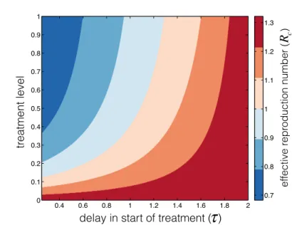
1), then increasing the delay increases Rc, and increasing the treatment rate decreases Rc. To illustrate the amount of delay we can afford for a given treatment rate to reduceRc below 1 (as a condition for disease eradication), we plotted the contours ofRc as a function of the delay in start of treatment (τ) and the treatment level (1−q(n)), whenR0= 2 (Figure 2) for influenza-like parameters. Note that the treatment level in this case is 1−q(n) = 1−e−(n−τ)θ. As shown in Figure 2, a higher level of treatment is required for Rc <1 as the delay for start of treatment increases. However, when the delay exceeds
0.4 0.6 0.8 1 1.2 1.4 1.6 1.8 2 0
0.1 0.2 0.3 0.4 0.5 0.6 0.7 0.8 0.9 1
0.7 0.8 0.9 1 1.1 1.2 1.3
treatment level
τ
delay in start of treatment ( )
R
c effective reproduction number ( )Fig. 2 Dependence of the effective reproduction number on the delay in start of treatment and the level of treatment with R0 = 2. Parameter values used for this simulation are:
p = 0.6,δA = 1/14, δU = 1/7,δT = 0.4,γ = 1/(70×365),µE = 1/1.25,µA = 1/4.1, µU = 1/2.85, µT = 1/1.35, dU = 0.002,dT = 0.001,βS0 = 0.84753, and n = 2. The treatment rateθwas varied in the range 0−5 andτwas varied in the range 0.25−2 [1].
approximately 1 day,Rccannot be reduced below 1 even with 100% treatment level, indicating the importance of early treatment in the control of disease.
In conclusion, as shown in our global analysis of the system, the delay term (τ) plays an important role in determining the possibility of disease control, which is reflected in the value of the effective reproduction number (Rc). As also demonstrated in our previous studies [9, 18], the delay term can be re- garded as a control parameter in epidemic models. Apart from the theoretical aspects of the global dynamics, this control parameter could provide impor- tant information on the long-term disease dynamics; for example to minimize endemic states of drug-resistance with delay in start of treatment [9], or to reduce timelines for achieving disease control in vaccine-preventable diseases with optimal booster vaccine schedule [18].
Acknowledgements
GR was supported by ERC Starting Grant Nr. 259559, and by Hungarian Sci- entific Research Fund OTKA K109782. TK’s visit to Hungary was supported by JSPS Bilateral Joint Research Project (Open Partnership). SM acknowl- edges the support of the Natural Sciences and Engineering Research Council of Canada (NSERC). JW acknowledges the support of NSERC and the Canada Research Chairs program.
References
1. Alexander, M.E., Moghadas, S.M., R¨ost G. and Wu, J., A Delay Differential Model for Pandemic Influenza with Antiviral Treatment, Bull. Math. Biol. 70 (2008), 382–397.
2. Alexander, M.E., Bowman, C.S., Feng, Z., Gardam, M., Moghadas, S.M., R¨ost, G., Wu, J., Yan, P., Emergence of drug-resistance: implications for antiviral control of pandemic influenza. Proc. R. Soc. Lond. B 274 (2007), 1675–1684.
3. Brauer, F., Shuai. Z., van den Driessche, P., Dynamics of an age-of-infection cholera model. Math. Biosci. Eng. 10(5-6) (2013), 1335–49.
4. Brauer, F., Xiao, Y., Moghadas, S.M., Drug-resistance in an age-of-infection model, Math. Pop. Stud. (2017) in press
5. Cai, L. M., Martcheva, M., and Li, X. Z., Epidemic models with age of infection, indirect transmission and incomplete treatment. Discrete Contin. Dyn. Syst. Ser. B, 18(9) (2013), 2239–2265.
6. Diekmann, O., Heesterbeek, J.A.P., Mathematical Epidemiology of Infectious Diseases, Wiley, Chichester, 2000.
7. Hale, J. K., Lunel, S. M. V., Introduction to functional differential equations. Applied Mathematical Sciences 99, Springer, New York 1993
8. Hyman, J. M., Li, J., Infection-age structured epidemic models with behavior change or treatment. Journal of Biological Dynamics, 1(1) (2007), 109–131.
9. Knipl, D., R¨ost, G., Moghadas, S.M., Population dynamics of epidemic and endemic etates of drug-resistance emergence in infectious diseases, PeerJ 5 (2017), e2817
10. Kermack, W.O., McKendrick, A.G., Contributions to the mathematical theory of epi- demics: Part I, Proc. R. Soc. Lond. A 115 (1927), 700–721.
11. Magal, P., McCluskey, C.C., Webb, G., Lyapunov functional and global asymptotic stability for an infection-age model, Appl. Anal. 89 (2010) 1109–1140.
12. McCluskey, C.C., Complete global stability for an SIR epidemic model with delay (dis- tributed or discrete), Nonlinear Anal. RWA., 11 (2010), 55–59.
13. McCluskey, C.C., Global stability for an SIR epidemic model with delay and nonlinear incidence, Nonlinear Anal. RWA., 11 (2010), 3106–3109.
14. McCluskey, C.C., Delay versus age-of-infection – Global stability, Appl. Math. Comput.
217 (2010) 3046–3049.
15. Moghadas, S.M., Bowman, C.S., R¨ost, G., Wu, J., Populationwide emergence of antiviral resistance during pandemic influenza. PLoS One 3 (2008), e1839.
16. Nelson, K.E., Williams, C.M., Graham, N.M.H., Infectious Disease Epidemiology, The- ory and Practice, Jones and Bartlett Publishers, 2004.
17. Qiu, Z., Feng, Z., Transmission dynamics of an influenza model with age of infection and antiviral treatment. Journal of Dynamics and Differential Equations, 22(4), (2010), 823–851.
18. Shoukat, A., Espindola, A., R¨ost, G., Moghadas, S.M., How the interval between pri- mary and booster vaccination affects long-term disease dynamics, BIOMAT 2016 Pro- ceedings (in press), World Scientific 2017
19. Smith, H. L., Monotone semiflows generated by functional differential equations, J. Diff.
Eqns., 66 (1987), 420–442.
20. Vargas-De-Le´on, C., Esteva, L., Korobeinikov, A., Age-dependency in host- vector mod- els: The global analysis, Appl. Math. Comput. 243 (2014), 969–981.