Dynamical modelling and model analysis in neuroendocrinology

(1)

Dynamical modelling and model analysis in neuroendocrinology

Theses of the Ph.D. Dissertation

Dávid Csercsik Supervisor:

Gábor Szederkényi, Ph.D.

Scientiﬁc advisor:

Katalin Hangos, D.Sc.

Péter Pázmány Catholic University Faculty of Information Technology

Budapest, 2010

(2)

(3)

Tartalmi kivonat

Dinamikus modellezés és modellanalízis a neuroendokrinológiában Ezen disszertáció elsődleges célja hogy az utóbbi évtized biológiai kutatásai során elért néhány fontos eredményt állapottér modellek segítségével a biológiai rendszer- elmélet keretei közé helyezzen. További cél, hogy egy, a biológiai modellezésben szé- leskörben elterjedt modellosztály identiﬁkálhatósági tulajdonságaival kapcsolatban eredményeket fogalmazzon meg. A tézisben részletezett és felhasznált matematikai modellek a közönséges diﬀerenciálegyenletek (ODE) körébe tartoznak, a modellek paraméterei optimalizációs eljárásokkal kerülnek meghatározásra.

Elsőként egy, a gyors (G protein csatolt), és lassú (β-arresztin csatolt) jelát- vitelhez kapcsolódó modell kerül bemutatásra. A javasolt modell alkalmas a két konvergens, de kvalitative különböző jelátviteli útvonal kölcsönhatásának, emellett a jelátvitel RGS és ERKP függő szabályozási módjainak leírására. A modell szimu- lációs eredményei az eredő G-protein függő és független ERK dinamika tekintetében jó egyezést mutatnak a kísérleti megﬁgyelésekkel.

Másodsorban, míg a Hodgkin-Huxley típusú modellek osztálya széles körben elterjedt, és domináns az elméleti idegtudomány irodalmában, közismertek az olyan tanulmányok, melyek ezen fontos modellosztály identifikálhatósági tulajdonságainak analízisét tűznék ki célul. Ebből kifolyólag egy Hodgkin-Huxley típusú feszültség- függő ioncsatorna identifikálhatósági tulajdonságait vizsgáltam voltage clamp mérési módszert feltételezve. Az identifikálhatósági eredmények tükrében egy új identifiká- ciós eljárást javaslok, mely a paraméterbecslési probléma dekompozícióján alapul.

A vizsgálat eredményei közvetlenül alkalmasak új kritériumok megfogalmazására a voltage clamp mérési eljárások tervezésének tekintetében.

Harmadrészt, a dolgozat a GnRH neuronok modellezésének és paraméterbecs- lésének kérdéseit vizsgálja egy egyszerű, egy komparttmentel rendelkező Hodgkin- Huxley típusú elektroﬁziológiai modell segítségével, mely hypothalamikus szeletben található GnRH neuronok voltage clamp görbéinek és a current clamp görbék leg- fontosabb tulajdonságainak (nyugalmi potenciál, depolarizációs amplitúdó, akciós potenciál utáni hiperpolarizáció, átlagos tüzelési frekvencia ingerlő áram hatására) reprodukciójára képes. A modell paramétereinek változtatásával, ami a nyugalmi potenciál emelkedéséhez vezet, a modell képessé válik a burst-ölésre. Vizsgálatra kerül a különféle paraméterek hatása a burst hosszára.

(4)

Abstract

Dynamical modelling and model analysis in neuroendocrinolgy The primary goal of this dissertation is to put certain importanat recent biological results of neuroendocrinology into the framework of systems biology by constructing and using dynamic state-space models. A further aim is to provide results corresponding to the identiﬁability properties of a system class widely used in biological modelling. The models detailed in this thesis are ordinary diﬀerential equation (ODE) models, the parameters of which are determined via optimization methods.

At ﬁrst, a model is provided for the description of convergent signaling pathways corresponding to rapid (G protein coupled) and slow (β-arrestin coupled) transmission. The proposed model is able to describe the interaction of the two convergent, but qualitatively diﬀerent signaling mechanisms, as well as the RGS and ERKP mediated regulation of signaling. The simulation results show that the model gives rise to an acceptable qualitative approximation of the G protein dependent and independent ERK activation dynamics that are in good agreement with the experimentally observed behavior.

At second, while the application of the Hodgkin-Huxley model class is widespread and dominant in the literature of computational neuroscience, there is a lack of articles, which aim at the analysis of the identifiability properties of this important system class. Motivated by this issue, the identifiability properties of a single Hodgkin-Huxley type voltage dependent ion channel model under voltage clamp circumstances are analyzed. Based on the results of identifiability analysis, a novel identification method is proposed, which is based on the decomposition of the parameter estimation problem in two parts. The results of the analysis are used to formulate explicit criteria for the design of voltage clamp protocols.

Thirdly, problems related to the modelling and parameter estimation of GnRH neurons were investigated. A simple, one compartment Hodgkin-Huxley type electrophysiological model of GnRH neurons is presented, that is able to reasonably reproduce the voltage clamp traces, and the most important qualitative features in the current clamp traces, such as baseline potential, depolarization amplitudes, sub- baseline hyperpolarization phenomenon and average ﬁring frequency in response to excitatory current observed in GnRH neurons originating from hypothalamic slices.

Applying parametric changes, which lead to the increase of baseline potential and enhance cell excitability, the model becomes capable of bursting. The eﬀects of various parameters to burst length are analyzed.

(5)

Notation and Acronyms

Notation of the variables and currents of the GnRH neuronal model

V membrane potential IA A-type potassium current

IK delayed rectiﬁer potassium current IM non-inactivating potassium current IT low voltage activated Ca²⁺ current

IR R type high voltage activated Ca²⁺ current

IL L type (slowly inactivating) high voltage activated Ca²⁺ current IleakN a sodium leak current

IleakK potassium leak current

(9)

Acronyms

AP Action potential

APPS Asynchronous parallel pattern search

CC Current clamp

DAP Depolarizing afterpotential E2 Estradiol

ERK Extracellular regulated kinase FSH Follicle-stimulating hormone GDP Guanosine-diphosphate GFP Green ﬂuorescent protein

GnRH Gonadotropin releasing hormone GPCR G protein-coupled receptor

GRK G protein-coupled receptor kinase GTP Guanosine-triphosphate

HH Hodgkin-Huxley HVA High voltage activated LH Luteinizing hormone LVA Low voltage activated

MAPK Mitogen activated protein kinase

MAPKP Mitogen activated protein kinase phosphatase ODE Ordinary diﬀerential equation

P4 Progesterone (P4)

RGS Regulators of G protein signaling VC Voltage clamp

(10)

Chapter 1 Introduction

Systems biology is an emerging interdisciplinary branch of science that aims at studying and computationally describing the interactions and interaction networks in biological systems [14, 17]. The models resulting from this approach can be used to explain dynamical mechanisms and phenomena, and for gaining predictions corresponding to the behavior of the system of interest.

To increase the clinical relevance of such models, one has to use sub-models based on as up-to-date biological information as available, and reduce the role of empirical and phenomenological approaches everywhere where the biological knowledge makes it possible.

The work reported in this thesis presents contributions to systems biology in the above sense: two chapters (2. and 4.) focus on systems biology models corresponding to neuroendocrinology [106], and one chapter (3.) focuses on methodological issues, especially mathematical (identiﬁability) properties of a model class (Hodgkin-Huxley type models) widely used in systems biology.

Motivation: Complex nonlinear elements in the female reproductive neuroendocrine system. Probably one of the most important known complex biological systems is the female reproductive neuroendocrine system. Here the buzzword complex [161, 42] corresponds not only to the high number of interacting elements and the high number of interactions (see Appendix A), but also to the special highly nonlinear nature of the observed dynamics.

The neuroendocrine cells in the hypothalamus secrete Gonadotropin releasing hormone (GnRH) in a pulsatile way [166], with GnRH pulse frequency varying on the scale of 8-240 minutes. The anterior pituitary, in response to GnRH, secretes hormones as well in a pulsatile way to stimulate the growth and development of ovarian follicles: Follicle-stimulating hormone (FSH) and luteinizing hormone (LH).

In addition to some other regulation mechanisms, the ovarian hormones feed back to the hypothalamus and also to the pituitary.

Via the multiple feedback loops connecting these endocrine and neuroendocrine tissues, the system of hypothalamic, ovarian and pituitary hormones together with morpological changes in the ovary regulate and maintain the menstrual cycle in adult women. Although cycles are usually between 25 and 30 days apart, but a woman’s normal cycle can range anywhere from 22-40 days long.

(11)

One of the most exciting challenge of the reproductive neuroendocrinology is to map the connections between these time scales of weeks and minutes (millisec- onds, if considering neuronal activity). Many results point to the assumption, that the understanding of this complex dynamics can not be done without the help of computational models [16, 21, 57, 62, 61, 129].

The aim of this work, however, is not to describe the whole reproductive neuroendocrine system, but to focus on some important interactions and elements, and create mathematical descriptions (computational models) for them, which include the paradigms of recent biological ﬁndings of the ﬁeld, and try to analyse and estimate them by using methods and tools of modern systems and control theory.

Especially the issues of key elements in the GnRH system are addressed: the G protein signaling, which is the mechanism via the hormone acts on the gonadotropin cells in the pituitary, and the GnRH neuron, which is responsible for the synthesis and secretion of this important neuropeptide.

β-arrestins and slow transmission: New aspects of signaling. Signaling through G protein-coupled receptors (GPCRs) is a well known mechanism of information transmission in intercellular communication (see later section 2.1). However, the operation of the intracellular pathways, which are connected to these receptors, are not yet fully understood, and in the recent decade signiﬁcant new biological mechanisms related to these pathways have been identiﬁed.

The most widely accepted classic paradigm of signaling until the 2000s has been that the significantly important elements which contribute to information transfer into the internal system of the cell are the α and βγ subunits of G proteins (see the review [104]). This paradigm was in good agreement with the classical concept of drug efficacy in the context of receptor-occupancy theory where the efficacy is considered as an intrinsic property of the ligand-receptor pair [52].

One of the most important main targets of the intracellular pathways aﬀected by G protein related signaling is the family of MAPK/ERK cascades [73, 90, 177], which play a central role in the intracellular signaling network. Proteins called G protein-coupled receptor kinases (GRKs) are able to rapidly terminate this signaling response via phosphorylating the receptor, typically on its cytoplasmic tail [128].

Following phosphorylation, β-Arrestins bind the receptor, which blocks further G protein-initiated signaling.

In recent years it has been shown thatβ-Arrestins not only take part in receptor desensitization [50], but form an endocyctic protein complex, which initiates a G protein independent regulation of ERK [36, 113, 127, 8, 10]. The recognition, that a single receptor acts as multiple source of signaling pathways and various drugs binding to this receptor might differentially influence each of this pathways (in contrast to pathway-specific drugs), led to the reassessment of the efficacy concept [52].

These biological ﬁndings opened a way for dynamical models [106], which are able to describe the interaction of the two convergent, but qualitatively diﬀerent signaling mechanisms. Section 2.2 is addressing this issue.

(12)

Identifiability properties of the Hodgkin-Huxley model class The HH (Hodgkin-Huxley) modelling formalism [71] of membrane currents and cell electrophysiology is the most widely used framework for the purpose of modelling excitable cells. The dynamical descriptions of neuronal behavior, ranging from the fundamen- tal theoretical principles [76, 77, 78] to the wide range of applications with special focus [136, 93, 133, 18, 46], are predominantly based on this model class.

Although several articles have been published which are focusing on parameter estimation problem in the case of HH based models under various assumptions (see [145, 144, 165, 148, 102, 74]), there is a lack of literature data which address the identiﬁability properties of such models.

Furthermore, there is a lack of a well grounded parameter estimation method that relies on the results of the identiﬁability analysis, and that can handle the possibly appearing identiﬁability problems.

Therefore, the aim of my work reported in this thesis was to provide a rigorous formal identiﬁability analysis of a simple Hodgkin-Huxley type ion channel model, interpret the results, and to provide a parameter estimation method which takes into account the arising possible identiﬁability issues.

Electrophysiological properties of GnRH neurons revealed through trans- genics and GFP tagging. As mentioned before, GnRH neurons govern important central role in the control of the reproductive neuroendocrine system. With the application of cell marking based on the green ﬂuorescent protein (GFP) and transgenic mice, the targeted measurements and electrophysiological experiments on GnRH neurons became available [67, 142]. Another possibility for gaining measured data is the application of "immortalized" GnRH neurons [119, 162], so called GT1 cells. Since these methods became widespread, the electrophysiological features of this important neuroendocrine cell have been studied extensively both experimentally and also several mathematical models have been constructed to explain the underlying mechanisms of their properties.

Until now, the mathematical models corresponding to GnRH neurophysiology were based mainly on data collected from immortalized GT1 cells. The behavior of these cells (eg. firing frequency, depolarization magnitudes) is significantly different compared to GnRH neurons in hypothalamic slices, which exhibit probably more common properties compared to in-vivo GnRH neurons.

However, in recent years, based mainly on the GFP tagging method, signiﬁcant amount of experimental data has been published on the electrophysiology of GnRH neurons [67, 138, 35, 80]. These articles, together with the possibility of targeted measurements can serve as a good basis for the synthesis of an electrophysiological model of the GnRH neuron, which is able to take into account as much as possible from the up-to-date biological knowledge corresponding to the ion channels and dynamics of this unique neuroendocrine cell.

The above motivating facts let us try to construct a simple Hodgkin-Huxley type dynamical model of GnRH cell electrophysiology based on literature data published on its various ionic currents, and estimate its parameters based on GFP based whole cell patch clamp recordings.

(13)

The structure of the thesis is as follows. In chapter 2 the biological background of G protein andβ-Arresitn coupled signaling is summarized, and the corresponding dynamical reaction kinetic model is described. Chapter 3.1 introduces the class of Hodgkin-Huxley type models of ionic currents and neuronal electrophysiology, analyses the identiﬁability properties of one such channel under voltage clamp conditions, and provides a parameter estimation method based on the results of identiﬁability analysis. Chapter 4 describes the dynamical neuronal model of GnRH electrophysiology. The possible applications and future perspectives are described in chapter 6. Appendix A gives a summary about the biology and interactions of the female reproductive neuroendocrine system. Appendix B descibes simulation results corresponding to a subsystem of the model described in 2. Appendix C details the procedure of electrophysiological recordings of the GnRH neurons. The mathematical details of parameter estimation, and estimated parameters of the GnRH neuronal model can be found in Appendix D.

(14)

Chapter 2 Dynamic models of intracellular

signaling pathways: rapid and slow transmission

In this chapter, a dynamic computational model is presented in the form of ordinary diﬀerential equations (ODEs), which describe the interplay of rapid (G protein coupled) and slow (β-arrestin coupled) transmission in the signaling process of ERK activation. At ﬁrst, in section 2.1, the biological background is detailed, then the model concepts, model development (section 2.2), model simulation results (section 2.3) and conclusions (section 2.4) are presented.

2.1 Rapid (G protein dependent) and slow (β -arrestin dependent) transmission

Diverse signaling molecules, including neurotransmitters, hormones, phospholipids, photons, odorants, taste ligands and mitogens, bind to their speciﬁc G protein- coupled receptors (GPCRs), also known as seven-transmembrane receptors (7TMRs), in the membrane of the target cells, which subsequently interact with their respective G proteins to induce a cascade of downstream i.e. intracellular signaling.

The G proteins are heterotrimeric signaling molecules composed of three subunits,α,β andγ, which dissociate upon receptor-induced exchange of GDP for GTP on theα subunit (Gα) to form a free Gα and a dimer of Gβγ subunits [60, 59, 114].

Many isoforms of these subunits have been cloned in the past years and have been classiﬁed into four groups according to the subtype of their α subunit: Gαs, Gαi, Gαq and Gα12. All these Gα subunits, as well as the dissociatedβγ subunits, and other receptor-interacting proteins are capable of initiating diverse downstream signaling pathways via second messenger molecules, such as cyclic AMP, cyclic GMP, inositol triphosphate, diacylglycerol, and calcium.

Activation of the signal induced by the GPCR depends on the rate at which ligand-bound receptor catalyzes exchange of GDP for GTP on the Gα subunit.

Following exchange, GTP-bound Gα dissociates, at least partially, from both the receptor and Gβγ complex. The length of time that GαGTP andGβγ can interact

(15)

with eﬀectors is determined by the rate at which Gα hydrolyzes GTP to GDP.

Following hydrolysis, inactive GαGDP bindsGβγ with high aﬃnity, and terminates Gβγ signaling. GTPase-activating proteins (GAPs) speed up the hydrolysis of GTP byGα [174]. In this work Gβγ signaling events are not examined.

The novel concept of slow transmission via β-arrestins has already been mentioned in section 1. Following GPCR activation, the ligand-bind receptor can be phosphorylated by GPCR kinases (GRKs). As described for eg. in [9, 8, 7] in the case of dopamine receptors, β-Arrestins bind to the receptors after phosphorylation to uncouple them from G proteins and participate in the recruitment of the endocytic protein complex, thus leading to an attenuation of GPCR signaling.

On the other hand, the signaling complex composed of the ligand, the receptor, β-Arrestin2, and PP2A can dephosphorylate the protein Akt on the site Thr308, and initiate a G protein independent signaling cascade. Furthermore, an another signaling complex binding to the phosphorylated receptor composed of β-Arrestin, ERK1/2, Raf-1 and MEK can initiate ERK activation [37]. The later case, leading to the β-Arrestin dependent activation of ERK, will be in the focus of this study.

Together, the G-protein and β-arrestin coupled pathways form a signaling network convergent to the central target kinase ERK.

Another important mechanism contributing to the dynamics of signaling is the feedback regulation, about which there are only a few models available in the literature [94, 176]. At the same time, eﬀorts to take into account the β-Arrestin dependent slow transmission as a second pathway convergent to G protein signaling is also not prevalent either in literature. The mechanisms of the regulation of G protein signaling are described in section 2.2.4 in detail.

2.2 Model developement

Much effort has been made nowadays to find plausible mathematical models for the description of the general dynamics of GPCR activation [1, 168, 169, 167], ligand efficiency [107, 25, 85] and receptor desensitization [143] in order to analyze signaling dynamics, and lay down the fundamentals of dynamical pharmacology [3].

To join the above mentioned efforts, the aim of this chapter is to propose a simple (in a sense minimal) reaction kinetic model and the implied equations for G protein signaling, based on biochemical and physiological observations collected about cell signaling pathways corresponding to a simplified model of fast-, and slow- transmission as well as the regulation of G protein signaling that is able to reproduce the downstream activation pattern (like ERK or Akt) recently described qualitatively in [37]. Our modeling effort is directed towards describing the dynamics, i.e.

the time evolution of the key components participating in G protein dependent and independent signaling. This may enable us to analyze cellular activation in the case of parallelly or competitively acting agonists and apply control theoretic methods for ﬁnding optimal drug dosing strategies in the future.

Three model variants will be developed. The basic model described in 2.2.1 is able to describe ligand binding, and the cycle of Gα GTP activation, deactivation and reactivation by the ligand-bound receptor. Thereafter, in section 2.2.3, we will

(16)

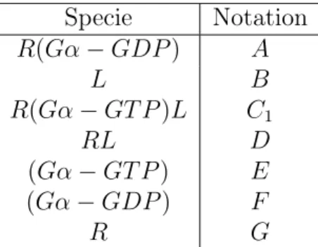
Table 2.1: Notations of species in the basic model Specie Notation

R(Gα−GDP) A

L B

R(Gα−GT P)L C1

RL D

(Gα−GT P) E (Gα−GDP) F

R G

extend our model with the reactions describing receptor phosphorylation by GRKs (G protein coupled receptor kinases), which is a key issue of the slow transmission process. Afterwards, in 2.2.4 we extend the model with the reactions describing the two convergent pathways of ERK activation, and the RGS and ERKP-mediated negative regulation of G protein signaling.

We aim at constructing a model in strict reaction kinetic form (governed by the mass action law), in order to stay in a model class for which the deficiency-based multistability-related results of Feinberg et al. [44, 31, 32] can be applied in the future. These results provide very strong theorems about qualitative behavior of reaction kinetic systems, based only on the structure of the reaction network, independently of its parameters. Furthermore, these and other [151, 152] multistability- related results offer the possibility to explain interesting physiological phenomena related to typical dynamic, pulsatile intercellular signals, for example, in the case of GnRH-affected gonadotropine cells [164], or dopamine-affected prolactin cells [12].

2.2.1 The basic reaction structure of the G protein signaling mechanism

The most simple reaction kinetic model of G protein signaling is constructed in this subsection, which is able to describe ligand binding, Gα activation, deactivation and reactivation. Furthermore, the model contains the Gαuncoupled ligand bound receptor that enables to extend the model with slow transmission related reactions in the following sections.

In order to simplify the form of the equations, the notations in Table 2.1 for species is introduced, with the notation Ci used for complexes.

For the development of a simple mathematical model of basic G protein signaling, the reaction scheme depicted in Fig. 2.1 is used. In the reaction schemes, the notation is the following: Arrows between components deﬁne transformations, and arrows pointing to arrows denote enzymatic catalysis (see the later reaction schemes).

It can be clearly seen from the reaction scheme in Figure 2.1 that the model does not describe active and inactive receptor forms, as for example the models detailed in [25, 143]. The reason for this lays in the fact that in this study the properties

(17)

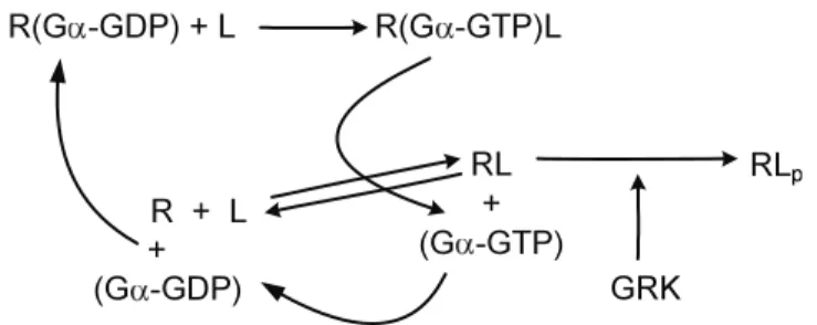
R(G -GDP) + L R(G -GTP)L

(G -GTP) + RL (G -GDP)

R + L +

Figure 2.1: The basic reaction scheme of G protein signaling: The receptor (R) binds the ligand (L), and induces GDP -> GTP exchange. Thereafter the GαGTP subunit dissociates, and after a while the GTP is hydrolyzed to GDP. After this, the Gα GDP subunit can reassociate with the ligand bound receptor.

of the ligand corresponding to achieve conformational changes in the receptor are not of primary interest, but the qualitative features of the two (G protein dependent and independent slow transmission) signaling pathways, and the feedback regulation of signaling will be in the focus. According to this aim, it can be assumed that conformation change of the receptor always appears after ligand binding, and is always followed by GDP/GTP exchange on the α subunit.

It is important to note that the primary input of the model is the ligand concentration on the cell surface. Processes aﬀecting the concentration proﬁle of the ligand such as degradation and reuptake, may be taken into account via the term Lenv in eq. 2.5. The Gα−GT P, and later, in the case of the extended model, the ERK activation corresponds to the output of the system.

2.2.2 The basic model

The basic model describes a cell together with the cell surface, and the only compo- nent for which the system is open, is the ligand. This can be understood as the eﬀect of the cell’s environment that inﬂuences the ligand concentration on the cell surface (if the ligand concentration in the environment rises, the ligand concentration on the cell surface will rise too).

For all other components, the system is closed. This can be described by the following conservation equations (see notations in Table 1):

• The conservation of G protein: [Gα^tot] = [A] + [C] + [E] + [F]

• The conservation of receptors: [R^tot] = [A] + [C] + [D] + [G]

• The conservation of the ligand: [L^tot] = [B] + [C] + [D]

The dynamic time-dependent or state variables of the system are the concentrations of the complexes, and the reactions in the system obey the mass action law.

(18)

Modeling assumptions

For the reactions, the following assumptions are made:

1. One molecule of ligand can activate one Gα − GDP-bound receptor, and phosphorylate the Gα−GDP to Gα−GT P.

2. The Gα−GT P subunit can dissociate from the ligand-bound receptor.

3. The recombination of the α and βγ subunits of the G protein is considered to be fast, and so the deactivation of the G protein is described by one reaction corresponding to the hydrolysis of GTP to GDP (as in [143]). Thus the Gβγ signaling, and βγ subunits are neglected.

4. The deactivated free Gα−GDP can associate with a free receptor and form a Gα−GDP-bound receptor complex, which can be activated again by one molecule of the ligand.

5. Phosphate required for phosphorylation reactions is present in a great excess.

6. We do not take receptor internalization into account. Results show that receptor internalization does not appear in many cases, for example in the case of prolactin cells [51].

State equations

The state or diﬀerential equations in the model will be derived from the reaction equations related to the reaction kinetic model formed by the chemical reactions.

The explicit derivation of the state equations is presented only in the case of the basic model structure of the G protein signaling mechanism. The method for deriving the equations from the reactions via the mass action law is the same in the case of the later models extended with slow transmission and the regulation of signaling.

The considered reactions (using the notation in Table 2.1) are as follows.

The binding of the ligand (L) by the (Gα −GDP)-bound receptor (R(Gα − GDP)), and receptor induced exchange of GDP for GTP on the Gα and the dissociation of Gα is described by the following reactions:

A+B k1⁺

GGGGGGB F GGGGGG

k1⁻

C1

k2⁺

GGGGGGB F GGGGGG

k2⁻

D+E (2.1)

The hydrolysis of Gα−GT P toGα−GDP is described as E k⁺3

GGGGGGB F GGGGGG

k⁻3

F (2.2)

Following hydrolysis, inactive GαGDP binds Gβγ and the free receptor G+F k⁺5

GGGGGGB F GGGGGG

k⁻5

A (2.3)

(19)

The dissociation of the ligand from the receptor is described in the form D k4⁺

GGGGGGB F GGGGGG

k4⁻

G+B (2.4)

The dissociation of the receptor and the ligand before reactivation of G protein is included to secure the ability of the ligand to escape from the cycle. Because the ﬁrst ligand binding reaction is assumed to be irreversible, and only the concentration of the free ligand is aﬀected by the input (the environment’s ligand concentration), there is no other way to describe the fall of the ligand concentration on the cell surface.

The above reactions imply the following diﬀerential equations by the mass-action law:

d[A]

dt = −k1⁺[A][B] +k1⁻[C1] +k5⁺[G][F]−k5⁻[A]

d[B]

dt = −k1⁺[A][B] +k1⁻[C1] +k4⁺[D]−k⁻4[G][B] +ks([Lenv]−[B]) d[C1]

dt = k1⁺[A][B]−k1⁻[C1]−k2⁺[C1] +k2⁻[D][E]

d[D]

dt = k2⁺[C1]−k2⁻[D][E]−k⁺4[D] +k⁻4[G][B] d[E]

dt = k2⁺[C1]−k2⁻[D][E]−k⁺3[E] +k⁻3[F] d[F]

dt = k3⁺[E]−k3⁻[F]−k5⁺[G][F] +k5⁻[A]

d[G]

dt = k4⁺[D]−k4⁻[G][B]−k5⁺[G][F] +k5⁻[A] (2.5) The term ks([Lenv]−[B]) corresponds to the input (u) of the system, in which u = L_env denotes the concentration of the ligand in the cell’s environment. Note that Lenv is a function of time in general.

Simulation results of the basic model can be found in Appendix B (10.1).

2.2.3 The extended model I: Receptor phosphorylation

If we want to take the concentration of phosphorylated receptor-ligand complex into account, which initiates the G protein independent slow transmission signaling, we have to extend our model with three more state-variables:

• The concentration of GPCR kinase - [GRK]

• The concentration of activated GPCR kinase and ligand bind receptor complex - [GRK −RL]

(20)

• The concentration of phosphorylated ligand bind receptor - [RL_p]

We assume that the concentration of phosphorylated receptors depends only on the concentration of GRK and on the concentration of ligand-bound receptors, which can be phosphorylated by GRK-s.

For the development of a simple mathematical model of receptor phosphorylation, the reaction scheme shown in Fig. 2.2 is used.

R(G -GDP) + L R(G -GTP)L

RL + (G -GTP) (G -GDP)

R + L +

RL

GRK

Figure 2.2: The reaction scheme of G protein signaling extended with receptor phosphorylation

2.2.4 The extended model II: Slow transmission and Regula- tion of signaling

In this section the further extended model is described, which includes the above detailed G-protein signaling model, the mechanism of receptor phosphorylation, slow transmission and the regulation of signaling.

As described in [37], β-Arrestins that bind the receptor after phosphorylation, can serve as scaﬀolding molecules that facilitate cell signaling to ERK (and also to other subgroups of MAPK proteins through MEK and Raf, as described in [90]).

The activation of MAPK cascades can be furthermore initiated by a small GTP- binding protein (smGP; RAS-family protein), which transmits the signal either directly or through a mediator kinase to the MAPK kinase (MAP3K or MAPK³) level of the MAPK cascades (MAPK-s are activated by MAP kinase kinases - MAPKKs -, which are in turn actiated by MAP kinase kinase kinases - MAP3Ks or MAPK³s).

As DeWire describes in [37], with si-RNA methods and the application of mutant receptors, it can be shown, that the resulting ERK phosphorylation (activation) is composed as a result of the activation induced by G proteins and the activation originated from β-Arrestin mediated slow transmission.

Experimental investigations show that the G protein-mediated ERK activity is maximal at 2 min after stimulation, and the β-arrestin2 mediated ERK activity is minimal until 10 min post-stimulation, but is responsible for nearly 100% of ERK signaling at times beyond 30 min [37].

It has also been shown [81, 89] that the regulators of G protein signaling (RGS) are basically the guanosine triphosphatase (GTPase)-accelerating proteins that specif- ically interact with G proteinαsubunits. RGS proteins enhance the intrinsic rate at which certain heterotrimeric G proteinα-subunits hydrolyze GTP to GDP, thereby

(21)

limiting the duration that α-subunits activate downstream eﬀectors. This activity deﬁnes them as GTPase activating proteins (GAPs).

These regulator proteins display remarkable selectivity and speciﬁcity in their regulation of receptors, ion channels, and other G protein-mediated physiological events [171]. Recent ﬁndings show that RGS proteins selectively regulate signaling by certain G protein-coupled receptors (GPCRs) in cells, irrespective of the coupled G protein [122].

Furthermore, RGS proteins can change the nature of the start and end of a signaling event, while leaving the intensity of the signal unchanged [174]. Results of the investigation of RGS protein functioning and regulation of G protein signaling in yeast can be found in [69, 40].

There are multiple RGS subfamilies consisting of over 20 diﬀerent RGS proteins.

RGS2 blocks Gqα-mediated signaling, a ﬁnding consistent with its potent GqαGAP activity.

MAPKs (including ERK) are feed-back regulated through map kinase phos- phatases (MAPKP orERKP), which are able to dephosphorylate MAPK-s [15, 94].

If RGS proteins were active unrestrictedly, they would completely suppress various G protein mediated cell signaling, as it has been shown in the over-expression experiments of various RGS proteins. Thus, physiologically the modes of RGS- action should be under some regulation. The regulation can be achieved through the control of either the protein function and/or the subcellular localization [75].

It can be assumed that RGS proteins (RGS2 and RGS3) are up-regulated via the phosphorylation of mitogen-activated protein kinases (MAPK or ERK) [94].

Extension of the reaction scheme

The further step in model development is to extend the model with the reactions describing the MAPK/ERK activation, and to take into account the RGS-mediated G protein feedback regulation, and ERKP mediated ERK auto-regulation. To make our model able to describe the signaling regulation process, we extend again the set of state variables (species) to obtain the set in Table 2.2.

(22)

Table 2.2: Notations for the ﬁnal model

Specie Notation Specie Notation

R−(Gα−GDP) A (Gα−GT P)−ERK C3

L B ERKp K

R−(Gα−GT P)−L C1 RLp−ERK C4

RL D RGS L

(Gα−GT P) E ERKp−RGS C5

(Gα−GDP) F RGSp M

R G RGSp−(Gα−GT P) C6

GRK H ERKP N

RL−GRK C2 ERKp−ERKP C7

RLp I ERKPp O

ERK J ERKPp−ERKp C8

Modelling assumptions

1. We assume that β-Arrestin, PP2A and Akt is in great excess, and they bind rapidly to the receptor forming the signaling complex, which immediately acti- vates the second messenger cascade leading to the induction of ERK signaling.

2. The ERK signaling cascade (MAP3K, MAPKK, MAPK) is neglected in the case of G protein based signaling.

3. Furthermore, we suppose, that RGS proteins are activated by the active form of ERK [94].

The phosphorylation of the ligand-bound receptor by GRK is described by the following reaction:

H+D k6⁺

GGGGGGB F GGGGGG

k6⁻

C2

k7⁺

GGGGGGB F GGGGGG

k7⁻

H+I (2.6)

The dephosphorylation of the phosphorylated receptor is represented by the reaction I k⁺8

GGGGGGB F GGGGGG

k⁻8

D (2.7)

We describe the signaling process and regulation by the reactions described in Eqs. (2.1) - (2.7) extended by the following reactions.

• The ERK activation by(Gα−GT P)andRL_P throughβ-Arrestin is described by the reactions:

E+J k⁺9

GGGGGGB F GGGGGG

k⁻9

C3

k10⁺

GGGGGGB F GGGGGG

k10⁻

E+K I+J k⁺11

GGGGGGB F GGGGGG

k⁻11

C4

k12⁺

GGGGGGB F GGGGGG

k12⁻

I+K

(23)

• The ERK-mediated RGS activation and the regulation of G protein signaling by the GAP-activity of RGS is represented by

K +L k13⁺

GGGGGGB F GGGGGG

k13⁻

C5

k14⁺

GGGGGGB F GGGGGG

k14⁻

K+M M +E k15⁺

GGGGGGB F GGGGGG

k15⁻

C6

k⁺16

GGGGGGB F GGGGGG

k⁻16

M+F

• Finally, the following reactions are related to the deactivation of ERK and RGS:

K k17⁺

GGGGGGB F GGGGGG

k17⁻

J M k18⁺

GGGGGGB F GGGGGG

k18⁻

L

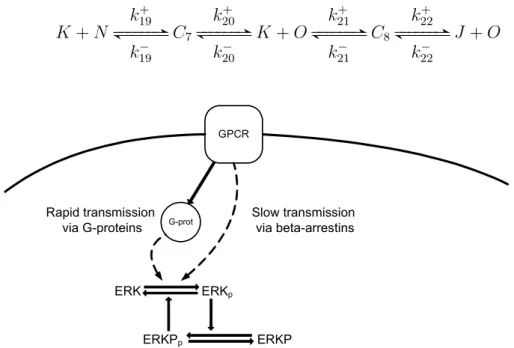
• If we also want to take into account the ERKP-mediated ERK feedback autoregulation shown in Fig. 2.3, we have to extend our system with the following reactions:

K +N k19⁺

GGGGGGB F GGGGGG

k19⁻

C7

k20⁺

GGGGGGB F GGGGGG

k20⁻

K+O k⁺21

GGGGGGB F GGGGGG

k⁻21

C8

k22⁺

GGGGGGB F GGGGGG

k22⁻

J+O

GPCR

G-prot

ERK ERKp

ERKPp ERKP

Slow transmission via beta-arrestins Rapid transmission

via G-proteins

Figure 2.3: The reaction scheme of ERK feedback autoregulation by ERKP: The ERK proteins can be activated either by the conventional G-protein coupled pathways or via slow transmission. In both cases the activation of ERK triggers the activation of the ERKP regulatory protein, which enhances the activation of ERK. The subscript _p denotes the active (phosphorylated) form of the proteins, the continual arrows indicate direct effect, and the dotted arrows indicate indirect effect through other molecules

• The deactivation of ERKP is described by the reaction O k23⁺

GGGGGGB F GGGGGG

k23⁻

N

(24)

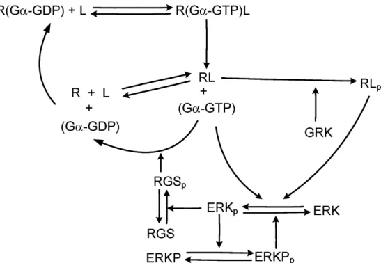
Figure 2.4: The reaction scheme of G protein signaling, ERK activation and regulation of signaling

The subscriptpin Figure 2.3 corresponds to the activated forms of the enzymes.

This mechanism is included in the resulting reaction scheme in Fig. 2.4.

Finally, the resulting reaction scheme in Fig. 2.4 summarizes the structure of all the above reactions. It is important to observe a large,RGS mediated and a small ERKP feedback loop, which implies a cascade structure.

2.3 Model verification

The models described in the above sections were veriﬁed by simulation. During the veriﬁcation process, the simulation results of the models were tested against theoretical expectations, and the simulation results of the extended model II were compared to published experimental data regarding the time evolution of ERK activation. This section describes and discusses these results.

2.3.1 Simulation results

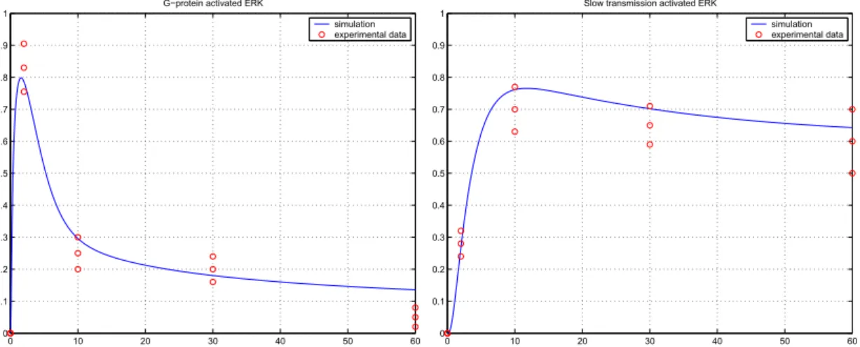
For the simulation of the extended model II, the parameters collected in Table 2.3 were used. The parameters were obtained via parameter estimation with MATLAB using the Nelder-Mead simplex algorithm for the best fit of experimental data of DeWire et al. [37, 105]. The right sub-figure of Figure 2.5 and both sub-figures of Figure 2.6 show averaged experimental values [105], and their empirical variances denoted by circles. For a good fit we expect the model to provide trajectories which remain in the intervals defined by the experimental deviations.

(25)

Table 2.3: Parameter set for the ﬁnal, extended model’s simulation Param. Value Param. Value Param. Value

k1⁺ 100 k9⁺ 5.3019 k17⁺ 6.2324 k1⁻ 100 k9⁻ 5.3019 k17⁻ 0 k2⁺ 120 k10⁺ 2.5539 k18⁺ 0 k2⁻ 0 k10⁻ 0 k18⁻ 0 k3⁺ 0.3170 k11⁺ 8.9418 k19⁺ 0.3791 k3⁻ 0 k11⁻ 8.9418 k19⁻ 0.3791 k4⁺ 1 k12⁺ 9.3924 k20⁺ 0.2354 k4⁻ 1 k12⁻ 0 k20⁻ 0 k5⁺ 1 k13⁺ 1.2696 k21⁺ 0.4 k5⁻ 1 k13⁻ 1.2696 k21⁻ 0.4 k6⁺ 0.6827 k14⁺ 1.2316 k22⁺ 0.4325 k6⁻ 0.6827 k14⁻ 0 k22⁻ 0 k7⁺ 0.3584 k15⁺ 5.9983 k23⁺ 0.015 k7⁻ 0 k15⁻ 5.9983 k23⁻ 0 k8⁺ 0.5 k16⁺ 6.6509

k8⁻ 0 k16⁻ 0

Note that the spontaneous deactivation of RGS protein was neglected in these ﬁnal simulation experiments, and so the parameters k⁺18 and k⁻18 were set to 0. The time interval of the simulations was 60 minutes in this case. The initial conditions were set to describe a fully deactivated cell with all signaling activations on the basal level.

We have to note that the sensitivity of the results with respect to certain parameters (eg. k1⁺, k⁻1, k2⁺) was not high enough to obtain an accurate estimated value.

A simple sensitivity analysis of the model is described in Appendix C.

It is important to note that if we wish to compare the resulting parameter values to the values found in the literature, we have to denormalize every concentration (which is hardly feasible due to imperfect information about intracellular protein concentrations), and modify the corresponding rate constants to achieve the same time patterns. This is why a simulation method with normalized concentrations has been used in our study to analyze only the qualitative features of the model structure.

The results of the simulations, i.e. the system responses are depicted in Figs.

2.5 and 2.6. In the left sub-ﬁgure of Fig. 2.5 the simulated Gα, RGS and ERKP -activation pattern can bee seen. Here again, the total activated ERK concentration is taken into account, which includes also the complexes, where the activated ERK acts as an enzyme (ERKP and RGS activation). In the case of other components, the concentration of the free element is depicted. In the case of ERKP the total active concentration is depicted (the sum of the free active enzyme and the complex with ERK). The reason for this is that the free active ERKP concentration is not very informative, as the enzyme immediately forms complexes with ERK.

(26)

0 10 20 30 40 50 60 0

0.2 0.4 0.6 0.8 1 1.2 1.4

Time [min]

Normalized concentrations

G−alpha GTP Activated RGS Activated ERKP

0 10 20 30 40 50 60

0 0.2 0.4 0.6 0.8 1

Time [min]

Normalized concentrations

activated ERK

simulation experimental data

Figure 2.5: Activation pattern of Gα−GT P, the corresponding regulators and ERK in the case of both transmission mechanism active. The circles on the second plot correspond to experimental results.

The Gα-activation pattern is strongly aﬀected by receptor phosphorylation and ERK-induced activation of RGS-proteins, which rapidly dephosphorylate theGα− GT P toGα−GDP.

0 10 20 30 40 50 60

0 0.1 0.2 0.3 0.4 0.5 0.6 0.7 0.8 0.9

1 G−protein activated ERK

0 10 20 30 40 50 60

0 0.1 0.2 0.3 0.4 0.5 0.6 0.7 0.8 0.9

1 Slow transmission activated ERK

Figure 2.6: G protein versusβ-Arrestin mediated signaling. The circles correspond to experimental results

In Fig. 2.6 we can see the ERK activation pattern corresponding to pure G protein dependent and G protein independent,RLp (β-Arrestin) mediated signaling.

The left sub-ﬁgure of Fig. 2.6 depicts the ERK activation in the case, when no slow transmission is taken into account. In the right sub-ﬁgure the G protein independent signaling is illustrated.

(27)

2.3.2 Discussion

If one wants to compare our simulation results with the experimental curves found in the literature, an important observation should be made. In several articles that reports on experiments (eg. [37]), the curves are normalized with the maximum concentration observed during the measurement. The reason behind this is, that in the case of many western-blot measurements, no information is available of the remaining inactive protein pool. These "actual maximum-normalized" curves can be easily derived from the data of our simulation results by re-normalizing the data with the actual maximum value of the concentration-curve. Unfortunately, a

"total quantity-normalized" curve can not be obtained from an "actual maximum- normalized" curve, if we do not have any information about the remaining, inactive protein pool.

The basic model described in 2.2.1 is able to describe the ligand-induced G protein activation in the cell, but is unable to describe receptor phosphorylation, the regulation of signaling. Furthermore, as described in Appendix B 10.1, the fast return of G protein activation to basal level after the stimulus also can not be described by this model, except if we suppose very fast spontaneous dephosphorylation of theGα−GT P to Gα−GDP. However, in this case a smaller part of the total G protein pool becomes activated, and a less signiﬁcant but non-zero steady-state is still present.

In the case of the extended model II, it can be seen in both Fig. 2.6 and 2.5 that the G protein activation and the G protein induced ERK activation has a pulsative maximum around 2 min, and is eliminated via the feedback of RGS activation. The G protein independent ERK activation, which can be related to the RLp concentration, has a slower rising period, and remains more stable during the simulation period.

As it can be seen in the second plot of Figure 2.5, the resulting activation pattern, which is in good agreement with experimental data, inherits the qualitative features of both pathways: The rapid maxima of ERK activation at 2-3 minutes can be related to the G protein dependent pathway, and the remaining tonic activation originates from the slow transmission pathway. Both the theoretical considerations and simulation results show that the resulting activation pattern of the second plot of Figure 2.5 is not the simple sum of the activation patterns depicted in Figure 2.6, because of the feedback mechanisms and other eﬀects.

We have to note again, normalized concentrations were used because of the lack of information about intracellular protein concentrations and in vivo reaction rate constants. This implies that the identiﬁed parameters can not be directly compared to literature data related to measurements with known concentrations. But the model fulﬁlls its main aim, and shows the required qualitative dynamic behavior and complexity for the description of the two-pathway regulated signaling system.

2.4 Conclusions

A simple, in a sense (regarding the number of reactions) minimal dynamic model of G protein dependent and independent signaling is proposed in this chapter. The

(28)

model focuses on the characteristic qualitative pattern of the time evolution of the key components this way enabling experimental veriﬁcation.

We have shown that if we take both ERK-mediated RGS and MAPKP feedback regulations into account, a qualitatively acceptable downstream behavior can be obtained in total ERK activation as well as in particular cases of G protein dependent and/or independent signaling.

Based on the simulation results presented here, we can conclude that modeling of slow transmission, RGS and MAPK-mediated regulation of signaling can be eﬃciently described using the framework of reaction kinetic systems, that may be essential when analyzing the dynamic behavior for physiological cell signaling. This type of model enables us to use the deﬁciency-based stability and multistability- related results of Feinberg et al. [44, 31, 32]. In addition, the determination of optimal time-dependent drug dosing may also be possible using control theoretic methods.

The proposed mathematical model could be an eﬀective tool to analyze the qualitative eﬀect of pathway selective drugs on signaling dynamics, for example Lithium in the case of dopamine-signaling [9], and to underline the importance of such medicines.

If the measurement or estimation of intracellular protein concentrations and rate constants were available, the model parameters could be re-estimated to quantita- tively fit experimental data, and be comparable to other literature results. Such an improvement of the model would be of great importance, since the relative concentrations of the proteins corresponding to the signaling system may vary with cell type and thus can give rise to qualitatively different signaling dynamics. This extension could open the way to study how the variation of cell stoichiometry of reactants can affect signaling kinetics.

(29)

Chapter 3 Identifiability and parameter estimation of a single

Hodgkin-Huxley type ion channel under voltage clamp measurement conditions

In this chapter some theoretical issues of Hodgkin-Huxley (HH) type models (the model class used later in Chapter 4) are addressed. in particular, the identifiability properties of a single HH type voltage dependent ion channel model under voltage clamp circumstances are analyzed. The elimination of the differential variables is performed, and the identifiability of various parameters is analyzed. As we will see, the formal identifiability analysis shows that even in the simplest case when only the conductance and the steady state activation and inactivation parameters are to be estimated, no identifiable pair from the three can be chosen.

In addition, a possible novel identification method is proposed, which is able to handle the arising identifiability problems. The proposed method is based on prior assumptions and on the decomposition of the parameter estimation problem in two parts. The first part includes the estimation of the maximal conductance value and the activation/inactivation parameters from the values of steady state currents obtained from multiple voltage step traces, utilizing the prior assumptions corresponding to the mathematical form of steady state functions. The use of steady state currents allows the estimation of the first parameter group independently of the other parameters. This parameter estimation problem results in a system of nonlinear algebraic equations, which is solved as an optimization problem.

The second part of the parameter estimation problem focuses on the parameters of the voltage dependent time constants, and is also formulated as an optimization problem. The parameter estimation method is demonstrated on in silico data, and the optimization process is carried out using the Nelder-Mead simplex algorithm in both cases.

The results of the chapter are used to formulate explicit criteria for the design of voltage clamp protocols.

(30)

3.1 The concept of identifiability

Once the model structure is ﬁxed (see later Eqs. (3.1)-(3.3) in our case), the next key step of the modelling process is parameter estimation the quality of which is crucial in later usability of the obtained model (see [109] and for e.g. the parameter estimation procedure detailed in chapter 4).

The identifiability properties of the system describe whether there is a theoretical possibility for the unique determination of system parameters from appropriate input-output measurements or not. Basic early references for studying identifiability of dynamical systems are the books [157, 158]. The study and development of differential algebra methods, that are used for identifiability analysis, contributed to the better understanding of important system theoretic problems [39, 47]. The most important definitions and conditions of structural identifiability for general nonlinear systems were presented in [110] in a very clear way. Further developments in the field include the identifiability conditions of rational function state-space models [115] and the possible effect of special initial conditions on identifiability [134].

Both the articles [102] and [165] realized the weaknesses of the conventional estimation algorithms, and provided improved methods for the estimation of HH models. Lee et.al. [102] proposed a new numerical approach to interpret voltage clamp experiments. As one of the main results of this article, it is stated, that all channel parameters can be determined from a single appropriate voltage step.

The aim of this chapter is to carry out a rigorous identiﬁability analysis in a simple case of the HH model class under voltage clamp measurement conditions in order to verify or falsify the above results related to parameter estimation of HH models.

3.2 Hodgkin-Huxley type mathematical modeling of membrane dynamics and ion channels

Hodgkin-Huxley (HH) models, which stand for the most widely used model class in computational neuroscience, are nonlinear electric circuit models, composed of parallel voltage dependent (and possibly voltage independent) conductances, which refer to various type membrane currents.

The basic modelling assumptions of the HH model, which are based on the kinetic description of the behavior of multiple voltage-dependent subunits [70], are evident and well formulated from the physical perspective. In contrast, if we analyze the model from the point of view of system theory, as a nonlinear state-space model (a system of nonlinear ordinary diﬀerential equations, ODE’s), several interesting questions arise, related not only to the bifurcation structure of the model [78, 55], but also to the identiﬁability properties of the system class [110].

The general HH model is based on the description of ionic currents in the following form:

I_i =g_im^p_i^mih^p_i^hi(V −E_i) (3.1) whereIiis the current of thei-th channel,miandhiare the corresponding activation and inactivation variables on the powersp_miandp_hi, which correspond to the number

(31)

of independent subunits of the voltage channel protein. V is the membrane voltage and Ei is the reversal potential of the corresponding ion.

The dynamics of the activation and inactivation variables are described by dmi

dt = (mi∞(V)−mi)/τmi(V), dhi

dt = (hi∞(V)−hi)/τhi(V) (3.2) where m_i∞(V) and h_i∞(V) denote the voltage dependent steady state values of activation and inactivation variables, and τmi(V) and τhi(V) denote the voltage dependent time constants.

In general, two basic measurement protocols are used for parameter estimation of neuronal models: the voltage clamp protocol, when the voltage is ﬁxed and the transmembrane currents are measured, and thecurrent clamp protocol, in which case an arbitrary value of injected current to the cell is ﬁxed. In the case of current clamp, the time evolution of the voltage can be calculated as a function of the membrane currents

dV

dt =−1 C(X

i

Ii) (3.3)

where in addition to the above detailed ionic currents with voltage dependent conductance, constant conductance leak type currents can also be taken into account.

In the case of voltage clamp, where the voltage is held constant, the only remaining diﬀerential variables are the activation and inactivation variables.

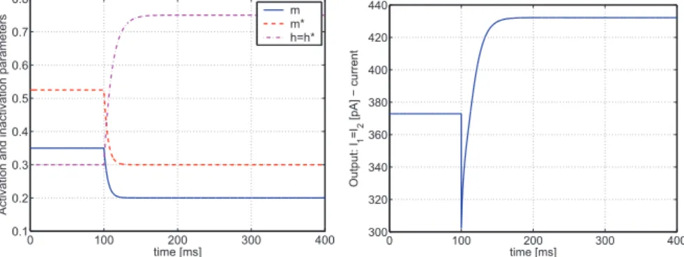
In the following, we analyze the identiﬁability properties of the most simple HH model, a single ion channel, under the assumptions of ﬁrst order activation and inactivation dynamics and voltage clamp measurement protocol.

3.2.1 A simple ion channel model

We consider a simple hypothetical ion channel with one activation (m) and one inactivation variable (h). The current, which is the measured variable under voltage clamp circumstances, is simply described by

I =gmh(V −E) (3.4)

whereV is the voltage,gis the maximal conductance, andEis the reversal potential of the corresponding ion. Both m and h are diﬀerential variables described by the equations

dm

dt = m∞(V)−m

τ_m(V) (3.5)

m∞(V) = µ

1 +exp

µV1/2m−V k_m

¶¶⁻¹

, k_m >0 (3.6) 1

τm(V) = µ

c_bm+c_amexp µ

−(V_{M axm}−V)² σ_m²

¶¶⁻¹

(3.7)

(32)

dh

dt = h∞(V)−h

τ_h (3.8)

h∞(V) = µ

1 +exp

µV1/2h−V k_h

¶¶−1

, k_h<0 (3.9)

1 τ_h(V) =

µ

c_bh+c_ahexp µ

−(V_{M axh}−V)² σ²_h

¶¶⁻¹

(3.10)

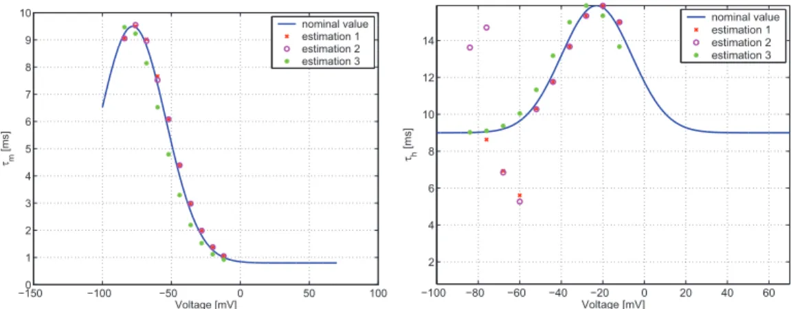
whereV1/2m,km,V1/2h, andkh are the parameters of the Boltzmann functions which describe the steady state activation and inactivation values. cbm, cam, VM axm, σm, cbh,cah,VM axh and σh denote the parameters of Gauss-functions which describe the voltage dependent time-constants.

We have to note that the approximation of the steady state values with Boltz- mann functions is not always valid, at it is described in [165]. However in the rest of this chapter we assume that this consideration holds. It can be said that in the literature the use of Boltzmann-type sigmoid functions is widespread for the description of steady-state values, but not exclusive (see e.g. [93]).

The description of the voltage dependent time constants in the literature is more diverse. In fact, the variability of time constant curves corresponding to various rate constant functions is described in [165]. In this study we will use standard Gauss functions, parameterized by cbm, cam, VM axm, σm, cbh,cah,VM axh and σh.

3.2.2 Voltage step protocol

An important version of the voltage clamp method is when the voltage, which is in this case the manipulable input (u) of the system, is held piecewise constant (V(t) =u(t) =V0 for t_k ≤t < t_k+1, k = 1, . . . , N). During each interval, the values of m∞, h∞, τm and τh can be considered as time-invariant parameters in addition to g and E. This implies that the non-polynomial nonlinearities of Boltzmann and Gauss functions (Eqs. (3.6), (3.7) and (3.9), (3.10)) are naturally eliminated from the equations, and the model will fall into the class of polynomial systems, which makes the application of eﬀective computer algebra based software tools (e.g.

DAISY [11]) possible for identiﬁability testing.

Under this circumstances will denote the voltage independent nature of the above parameters shortly by supressing the V argument, i.e. m^∞(V) =m^∞, τm(V) =τm, h∞(V) = h∞ and τ_h(V) =τ_h, with V =V0.

In this case, Eqs. (3.4-3.10) are simpliﬁed as follows:

I =gmh(V0−E) = gmh(u−E) (3.11) y=I, u=V0 =const.

dm

dt = m∞−m τm

, dh

dt = h∞−h τh

(3.12) where the model parameters are g, E, m∞, τm, h∞ and τh.