14-2 Rate Laws and Simple Mechanisms

CHAPTER FOURTEEN

KINETICS OF

GAS-PHASE REACTIONS

14-1 Introduction

The emphasis up to this point has been on the equilibrium properties of sub- stances in pure or solution form. The rate processes considered have been restricted to transport phenomena such as diffusion and conductance. Chemical kinetics is a more complicated subject than that of chemical equilibrium because time is now a variable in the description of the state of a system and because there may be more than one reaction path whereby reactants become products. The theory is difficult because such paths involve molecules in energetic and otherwise unusual states; these states can rarely be studied by themselves independently, so theoretical models contain assumptions which cannot be corroborated in detail.

There are three major facets to the study of chemical kinetics. The first might be termed the experimental side but involves not only the measurement of reaction rates but also their reduction to what we will call a rate law. ln chemical kinetics we retain the historic mass action rate law (Section 7-1) by expressing the rate R of a reaction at constant temperature as a function of the composition of the system,

R = ~ ^ d T = / [ ( A ) > ( B )'^{( C ) )} -^]- ⁽¹⁴"^1}

The complete function can be complicated, but it is often of the form

R = k(A)^x(B)y(C)^z - , (14-2)

where A, B, and C are reactants. This may come about either naturally or by deliberate choice of experimental conditions, such as having one reagent in great excess so that its concentration is constant. Thus if the complete rate law were either

R = 1 * ^ 3 ^{o r R} = *(A) + k'(A)(C),

it would reduce to one of the preceding type if (C) were constant; one could then 543

carry out a series of experiments in which the constant level of (C) was varied.

The constant k in Eq. (14-2) is called the rate constant, and the expression which gives R as a function of concentrations is the rate law. The first goal of the experi­

mental stage is then to devise and carry out experiments that will establish the algebraic form of a mass action type of expression for R and to evaluate the rate constant or constants that it contains. The next experimental stage is that of determining how such constants vary with temperature and with the nature of the reaction medium.

The second facet of chemical kinetics is that of reaction mechanism. It turns out that with few exceptions the fundamental act of chemical change involves just one or two molecules at a time; that is, elementary reactions in kinetics are nearly always unimolecular or bimolecular. The overall reaction that is being studied may, however, occur through a series of such elementary steps, which then gives the experimental rate law some complicated form. The steps, typically, will involve transient chemical species or reaction intermediates whose presence is not always independently provable. The reaction between H² and B r², for example, is considered to occur through hydrogen and bromine atoms as inter­

mediates, and steps in the overall reaction include Η + Br² = HBr + Br.

It is this detailing of the intermediate bimolecular steps constituting the path for the overall reaction that is known as the reaction mechanism. One uses mainly the experimentally observed rate law, but in general all available information, to infer a reaction mechanism that is consistent with the kinetics of the system. The study of reaction mechanisms is the final goal of the more chemically oriented investigator; the field can be a very controversial one because it has happened that two or more mechanisms, each equally capable of explaining the data, have each received strong partisan support.

Third, the theoretical study of elementary reactions is now highly developed.

It is concerned with the detail of how molecules approach each other, what their special requirements are for reaction—for example, with respect to energy—and with just how the crucial act of chemical bond making or breaking occurs. The two principal theoretical models of current importance differ considerably in flavor. If the elementary reaction is one of A with Β to give products, and we suppose that state [AB]* is that in which the two reactants have come together with the necessary energy and so on for reaction, but have not yet fallen apart into products, we can write

A + Β fci [AB]* ^ products. (14-3)

The first model, that of collision theory, deals with the rate at which A and Β can form [AB]* and thus emphasizes k², and, in its simpler form, ignores k_² so that [AB]* is considered always to go on to products. The second model, that of transition-state theory, treats [AB]* as being in equilibrium with A and B, so that the reaction rate is determined by the [AB]* concentration and by the fre­

quency or rate constant k^x.

The two models approach each other when pursued to a more sophisticated level, but each in its simple form has provided a framework or a language for qualitative explanations as to why a given reaction is fast or slow. Both are there­

fore presented.

Although chemical kinetics can be outlined as a unified general subject, as has been done here, when details are explored facets of the treatment of gaseous and

14-2 RATE LAWS AND SIMPLE MECHANISMS 545 solution systems tend to separate as distinguishable subfields. The three aspects just described develop different emphases and different bodies of empirical fact.

For this reason the material has been separated into two chapters. We first take up the subject of rate laws and their algebraic manipulation and then that of some important mechanisms of gas-phase reactions. The two major theories are next presented, with emphasis on their application to gaseous systems. Chapter 15 covers some of the experimental techniques special to solution systems and then proceeds to a discussion of how both collision and transition-state theory are modified in the case of solutions.

A rate law is conventionally presented in the form of Eq. (14-1), that is, as a differential equation, and the principal concern at the moment is with the mathe­

matical characteristics of specific functions / [ ( A ) , (B), (C),...], including their integrated forms. There is virtually no limit to the complexity of functions that may be encountered, and only the more important ones are taken up here. Also, we will consider only reactions that go to completion, deferring the more general case until Chapter 15.

A major category of rate laws is that for which R is given by an expression of the form of Eq. (14-2). We then speak of the order of the rate law as the sum of the exponents (x + y + ζ ···), the important cases being those of first- and second- order reactions, Although the rate law bears no a priori relationship to the chemical equation for the overall reaction, the stoichiometry of this last must always be kept in mind; this point will be illustrated in Section 14-2B.

A. The First-Order Rate Law

Suppose that the forward rate Rt of a reaction is found to depend only on the concentration of some reactant A.

The rate law is then

where Rt is the forward reaction rate. If the reaction goes to completion, then Eq. (14-4) provides the complete description of the rate behavior since R\>, the rate of the back reaction, is zero. Integration gives

14-2 Rate Laws and Simple Mechanisms

d(A)

= - * ( A ) (14-4)

and the overall reaction may be condensed to the form

A + other reactants products, (14-5)

or

ln(A) = — kt + constant. (14-6)

Thus a plot of ln(A) versus t gives a straight line of slope equal to —k⁹ as in

Fig. 14-l(a), where k is the rate constant, usually given in s e c^{- 1}.

It may be convenient to evaluate the constant of integration by setting (A) = (A)⁰ at t = 0. Equation (14-6) then becomes, in exponential form,

(A) = ( A )⁰e - « (14-7)

and the graphical appearance is illustrated in Fig. 14-1(b). A characteristic time is that at which (A)/(A)⁰ = \\ this is called the half-life t^1/2 of the reaction, and is very simply related to k:

1 A ) - \ = e-^M>'\.., In \ = ~kt^ut (14-8) (A)⁰ 2 - ' " ' 2

or

kt^ll2 = 0.6931. (14-9)

Thus either k or t^1/2 defines the rate of a first-order reaction. Note that if t = 2t^1/2, the effect is to double the exponential in Eq. (14-8), so that (A)/(A)⁰ = (J)² = J.

T i m e (units o f /^{1 / 2}) (a)

F I G . 14-1. The first-order rate law. (a) Plotted according to Eg. (14-6). (b) ( A ) / ( A )⁰ as a function of time, showing the constancy of ί1/2 .

In general, if t = n /^{1 / 2},

14-2 RATE LAWS AND SIMPLE MECHANISMS 547

(A) _ /ly

(A)⁰ (5) · (14-10)

This is illustrated in Fig. 14-l(b): (A)/(A)⁰ = \ a t r^{1 / 2}, J at 2t^1/2, £ at 3 f^{1 / 2}, and so on.

Example. It takes 10 m i n for a certain first-order reaction t o g o 2 0 % toward c o m p l e t i o n . W h a t are k a n d t^{l l 2} a n d h o w long s h o u l d it take for 75% reaction? B y E q . (14-7), ln(0.8) = - £ ( 1 0 ) , w h e n c e k = 0.0223 m i n "¹ a n d t^{l l 2} = 0.6931/0.0223 = 31.1 m i n . A t 7 5 % reaction, ( A ) / ( A )⁰ = 0.25 or i ; t h e required time is t w o half-lives or 32.2 m i n .

There is nothing unique about the time for half reaction—any other fraction could be picked.

Were w e t o speak o f t^xi^z, the analog o f Eq. (14-8) would be kt^x/^z = —In J, and in general if tx/r is the time for ( A ) t o drop t o the fraction 1/r o f its initial value,

ω ⁼ I ^{= E- MLLR KT =} _^{I n} I ^{( 1 4}.^{n )}

(A)o r r

and

(A)

(A)o

(τΓ·

^(14-12)

where n^r is the time expressed in multiples of t^xi^T. A n important feature o f an exponential function is then that if it takes a time t^Xj^r for ( A ) t o decrease by factor 1/r, then in a second such interval of time a further decrease by the same factor will occur, or an overall decrease o f (1/r)², and s o o n . A numerical illustration is given in Section 14-3.

It is sometimes useful t o take 1/r = 1/e, in which case tx\r is given the special symbol τ a n d is k n o w n as the mean lifetime for the reaction since it is, in fact, the average time elapsed before a molecule o f A reacts. Substitution into E q . (14-11) gives 1/e = e~^kT, o r —1 = — kr, whence

kr = 1. (14-13) The quantity τ can be shown t o be the mean lifetime as follows. F o r the m o m e n t let the mean

lifetime be denoted by f, which w e define by weighting each value of / by the amount of A present:

t =

J o o l c o , / d(A) _ [ ( A W * ] Jto00 (kt) er" d(kt)

i = 7 I - e -k\ \ + kt)U = \

k k Thus i is identical t o τ.

β. The Second-Order Rate Law

Consider the case where the overall order of reaction in Eq. (14-2) is found t o be two, that is (x + y) = 2, either because the rate is proportional t o (A)² or because it is proportional t o (A)(B). In the first case we can use Eq. (14-5) as giving the overall process, and write the rate law as

Rt = - ^ = A:(A)². (14-14)

We again assume that the reaction goes to completion, so that Rh is zero. Note that the rate constant k now has the dimensions of (concentration)^{- 1} ( t i m e )^{- 1};

time is usually given in seconds, and in the case of gases, concentration is commonly expressed in terms of partial pressure, so k might be in a t m o s p h e r e^{- 1} s e c o n d^{- 1}.

The integration of Eq. (14-14) is straightforward:

j ^ 1 = - jkdt or = kt + constant. (14-15)

As illustrated in Fig. 14-2(a), a plot of 1/(A) versus t gives a straight line, with intercept 1/(A)⁰ and slope equal to k, so that

m = jk

^+kt

-

^(,4

-

¹⁶⁾

One may again use the concept of half-life, and setting (A)/(A)⁰ = £ at r^{1 / 2} in Eq. (14-16) gives

2 - 1 = (A)⁰ kt^m or r^{1 / 2} = . (14-17)

However, unlike the case of a first-order reaction, the time for successive diminu- tions in (A) by a factor of one-half is not a constant, but doubles with each decre- ment. Thus /^{1 / 4} = 3/&(A)⁰ and t^1/8 = 7/k(A)⁰ , so that, as illustrated in Fig. 14-2(b), the first interval is r^{1 / 2}, the second 2 f^{1 / 2}, and so on.

F I G . 14-2. The second-order rate law. (a) Plotted according to Eq. {14-16). (b) ( A ) / ( A )0 as a function of time, showing the successive doubling of /^1/2.

14-2 RATE LAWS AND SIMPLE MECHANISMS 549

If the rate law is second order but of the form

R t = - ^ = fc(A)(B), (14-18) the reaction type becomes

a A -f bB + other reactants products. (14-19) We again assume that there is no back reaction, but note that Rt could equally

well be expressed in terms of d(B)/dt, from the stoichiometry of the reaction,

i m - m . (14.20)

a dt b dt ^v '

A notation that is convenient at this point is that of defining χ as the decrease in concentration in A at time t, χ = (A)⁰ — (A), and similarly, y = (B)⁰ — (B).

We then have

df(A) _ dx d(B) _ dy dt dt' dt dt

The simplest case is that for which b = a, so that the rate law becomes

£ = * [ ( A ) . - * ] [ ( B )⁰- , ] or m

- ^

^m

— -

^{r k d}

,

^(14-21)

On integrating, we obtain

( A ) o - (B)o'" ( A )¹

— t o fa

⁰[ ( B )⁰- x ] or

In |5M^- = [⁽A)⁰ - (B)⁰] kt. (14-22)

There are two special cases of interest. First, if (A)⁰ <^ ( B )⁰, then very little Β is consumed so that (B) is essentially constant and equal to ( B )⁰. The effect is that Eq. (14-18) reduces to the form

- =

[fc(B )oKA)

= fc^app(A), (14-23) or to the same form as the first-order rate law, Eq. (14-5).

Since fc^app is not a true rate constant but the product of k and the concentra­

tion (B)⁰ , it is customary to call Eq. (14-23) a pseudo-first-order rate law. This term is applied whenever a first-order rate expression has been obtained by virtue of some concentration or concentrations being held constant. The distinction is important to the mathematics of the situation, in that &^app will vary with ( B )⁰. Thus Eq. (14-23) gives the time rate law for a particular experiment, but not the full concentration rate law. The distinction can also be quite important in any

theoretical interpretation of the rate constant.

The second special case is that for ( A )⁰ = (B)⁰. Equation (14-22) becomes in­

determinate, and it is necessary (as always in such a circumstance) to return to the original differential equation. Since a = b, it follows that (A) = (B) at all times

during the reaction. Equation (14-18) therefore reduces to

or to Eq. (14-14).

These two special cases illustrate an important point for the experimentalist.

By choosing (A)⁰ <^ ( B )⁰, we reduce the rate law to a first-order one, and by choosing (A)⁰ = ( B )⁰, we reduce it to a much simpler mathematical form of a second-order rate law. Part of the art of experimental chemical kinetics lies in the designing of experimental conditions so that the mathematical complexity of the time rate law is reduced.

Example. T h e rate law for the reaction A + Β —* products is d(A)ldt = — k(A)(B) with k = 0.02 M "¹ m i n^{- 1}. W h a t percent o f A has reacted after 15 m i n if (a) ( A )⁰ = 0.1 Μ and ( B )⁰ = 0.3 M , (b) ( A )⁰ = ( B )⁰ = 0.1 M , and (c) if ( A )⁰ = 0.001 Μ and ( B )⁰ = 0.3 M ? (a) B y Eq. (14-22), ln[(0.3)(A)/(0.1)(B)] = (0.1 - 0.3)(0.02)(15) = - 0 . 0 6 , whence (A)/(B) = 0.3139.

Since (A)/(B) = (0.1 - *)/(0.3 - x), w e find χ = 8.49 x 1 0 "³ M , corresponding t o 8.49%

reaction o f A . (b) W e n o w use Eq. (14-16), which gives 1/(A) = 1/0.1 + (0.02)(15), whence ( A ) = 0.09709 Μ and the percent reacted is 2.91%. (c) T h e reaction is p s e u d o first order because of the great excess o f B , s o l n [ ( A ) / ( A )⁰] = -k^&vpt = - ( 0 . 0 2 ) ( 0 . 3 ) ( 1 5 ) = - 0 . 0 9 , whence ( A ) / ( A )⁰ = 0.9139, corresponding t o 8.61% reaction.

Note. T h e reaction stoichiometry might be 2 A + Β - > products, but with the rate still first order in ( A ) a n d in (B). W e w o u l d n o w write d(A)/dt = — 2&(A)(B) since it is customary t o define rate constant in terms of the reaction and in this case t w o m o l e s of A disappear per m o l e o f reaction. See Exercise 14-7.

W e return briefly t o the general case o f α Φ b, or t o Eq. (14-21). T h e rate law is n o w written d(A)ldt = ak(A)(B) since it is conventional t o define rate constants in terms of the process rather than in terms of any particular species. T h u s R = (1/a) d(A)jdt = (lib) d(B)ldt. E q u a t i o n (14-21) b e c o m e s

J = ak[(A\ - *][<B). - \ x \ (14-24)

which gives, o n integration,

In g^g = ^{W A} ) . - * ( B )⁰] kt. (14-25)

A g a i n , a suitable choice of experimental conditions can greatly simplify matters. If ( B )⁰/ ( A )⁰ is m a d e equal t o b/a, then Eq. (14-24) b e c o m e s

J = bk[(A)⁰ - xY or ^ = -bk(A)\ (14-26)

s o that the simpler form o f Eq. (14-14) has been regained, with &^{a P}p = kbja.

C. The Zero-Order and Other Rate Laws

The term "zero order" is applied to a reaction whose rate is independent of time, that is,

R = — ^ψ- = k (14-27) at

or

(A) = (A)⁰ - kt. (14-28)

14-3 EXPERIMENTAL METHODS AND RATE LAW CALCULATIONS 551

14-3 Experimental Methods and Rate Law Calculations

A. Use of Additive Properties

As stated earlier, an important goal of the experimentalist is that of establishing the rate law which governs a given reaction. The initial task is very similar to that in the study of chemical equilibrium—one needs some way of following the degree of reaction. As discussed in Section 7-3, one may quench or otherwise stop a reaction and then proceed at one's leisure to analyze chemically for reactants or products. However, very often some specific physical property of one or more of the species may be measured in situ, so that one may follow the reaction con­

tinuously as it proceeds. If one of the reactants has a characteristic light absorption, for example, the optical density of the solution may be monitored at a particular Such rate laws are more properly called pseudo-zero-order, since Eq. (14-27) gives the time dependence of (A) but cannot be the full description of the factors affecting the rate.

This point may be illustrated as follows. First, in photochemical reactions if the entire incident radiation is absorbed by the reacting species, then the rate of reaction will not depend on concentration and hence will be of zero order. However, the complete rate law is actually R = Ι&κβφ, where Tabs is the intensity of the absorbed light and φ is an efficiency factor called the quantum yield for the reac­

tion (see Section 18-4E); in the form written Tabs would be expressed as quanta of light per unit volume per second. Thus although the rate does not depend on (A), it does depend on Tabs ; at a sufficiently low concentration of A, Tabs will become proportional to (A), and the rate law will revert t o first order in (A).

Second, many examples of zero-order reactions occur in heterogeneous catalysis.

The situation is one in which the reaction takes place on the surface of the catalyst so that R = k'tisi, where θ is the fraction of surface covered by the adsorbed reactant and s/is the total catalyst surface area. If the concentration or pressure of A is large enough, θ = 1, and the reaction is zero order; at sufficiently low pressures, however, θ becomes proportional to (A) and the reaction reverts to first order. Note that R will depend on the amount of catalyst, that is, on the area s/, as well. See the Special Topics section for further details.

Experimental rate laws may be of some general order «, t h e simplest case of which is

" Τ

^{= k ( A r}

'

^{( 1 4}

"

^{2 9 )}

Integration gives

T^-lW^

^{= in}

-

^l)kt

'

⁽¹⁴

"

³⁰⁾

provided that η Φ 1. Some examples are the interconversion of ortho- and para- hydrogen, for which η = f, the formation of phosgene (CO + C l² = COCl²), for which η = f, and a variety of reactions for which η = 3.

wavelength. In the case of a gas-phase reaction the change in the total pressure may be used as a measure of the degree of reaction (provided the number of moles of gaseous products differs from that of the reactants).

These last two quantities, optical density and total pressure, are examples of additive properties 9 discussed in Chapter 3. There is a very useful relationship whereby 9 for a reacting mixture may be used to give the degree of advancement of the reaction. Consider the general reaction

aA + bB + · · = m M + « N + · · · . (14-31)

Initially A⁰ moles of A, B⁰ moles of B, and so on are present, and we have

= Α Λ + B ^^B + .... (14-32)

We now define ν as the degree of advancement of the reaction, where av is the number of moles of A reacted, bv the number of moles of Β reacted, and so on, and mv is the number of moles of Μ produced, nv is the number of moles of Ν produced, and so on. After some time t we then have

0>^t = [A⁰ - av\0>^h + [ B⁰ - bv]P^B + + mv&>^M + m0^ + ..., so that

- 0>^t = av0>^A + bv&^B + *·· - mv0>^M - ηι>0>^Ν . (14-33) At infinite time, or on completion of the reaction, ν has the value ν*,, and so

0>„ = [ A⁰ - av„]0>^A + [ B⁰ - feool^i + - + ^ O O ^ M + nv^ + ..., so that

- 9>^m = avjP^K + bva&s + mv„0>^M - nvjP* - - (14-34) and therefore

0

= ( 1 4"3 5 )

the term {a0*^A + b&^B + ··· — m£P^M — — ···) being a common factor to both Eqs. (14-33) and (14-34). Alternatively, we have

= 1 - — = r A \ rw ' (14-36)

^ o - ^ c o x v«, ( A) o- ( A ) «

We see that the second part of Eq. (14-36) is correct by writing (A)^t as [ A⁰ — av]jv and so on, where ν is the volume, and observing that the result simplifies to 1 — (W^co).

As a specific example, paraldehyde, ( C H³C H O )³, dissociates into acetaldehyde, the overall reaction being of the form

A = 3B.

The change in total pressure with time at 260°C is given in Table 14-1 and applica­

tion of Eq. (14-36), with 9 = P^TOT (total pressure), then gives PJPO.A , or the fraction of paraldehyde remaining (POO.A being zero in this case since the reaction

14-3 EXPERIMENTAL METHODS AND RATE LAW CALCULATIONS 553 T A B L E 1 4 - 1 . Thermal Dissociation of Paraldehyde

at 260°C

Time

(hr) (Torr) PA/PO.A

0 100 1.00

1 173 0.64

2 218 0.41 = (0.64)2

3 248 0.26 = (0.64)*

4 266 0.17 = (0.64)*

00 300 0.00

goes to completion). The results are plotted in Fig. 14-3, according to Eq. (14-6), and the linearity of the plot indicates that the reaction is first order. In Fig. 14-4, the data are also plotted according to Eq. (14-16), which tests for possible obedience to the second-order rate law, but the points now fall on a curved line. As indicated in the table itself, one could determine the first-order character directly by noting that ΡΑ/PQ.A drops by the constant factor 0.64 with each interval of 1 hr.

T i m e , hr

F I G . 14-3. The thermal decomposition of paraldehyde. Data plotted according to the first-order rate law.

8 r

I ι ι ι ι ι 1

0 2 4 6

T i m e , hr

F I G . 14-4. The thermal dissociation of paraldehyde. Data plotted according to the second-order rate law.

The rate law for the reaction is therefore

= -kP^A, dP^A

dt

and there are several ways in which k might be obtained. The slope of the line in Fig. 1 4 - 3 gives k = —[ln(O.l) — l n ( l) ] / 5 . 2 = 0 . 4 4 h r^{- 1}. Alternatively, t^{l l 2} is read from the graph as 1 . 5 7 hr, and by Eq. ( 1 4 - 9 ) , k = 0 . 6 9 3 / 1 . 5 7 = 0 . 4 4 h r "1. Finally, kt⁰.^6A = - l n 0 . 6 4 = 0 . 4 4 , and so k = 0 . 4 4 / 1 = 0 . 4 4 h r "¹.

B. The Isolation Method

The preceding subsection dealt with one very common method of determining an experimental rate law—that of fitting data to the integrated form of a specific rate law. This procedure is accurate and very satisfactory if the reaction rate is some integral order in a single reactant, or a second-order reaction in two reactants. If the data do not fit one or another simple integrated form, the number of more complicated possibilities rises rapidly, and the approach becomes increasingly less definitive, that is, the various more complicated integrated forms may not actually differ enough to allow a clear experimental distinction among them. At this point it becomes very useful to fix one or another concentration so as to isolate the dependence of the rate on each species in turn. One usually does this using a large excess of first one reactant and then another.

An illustration may be constructed as follows. The reaction

2 N O + H² = N²0 + H²0 ( 1 4 - 3 7 )

is known to obey the rate law dP^p

dt ^{= kP^QPH2}, ( 1 4 - 3 8 ) with k = 1 . 0 0 χ 1 0 ~⁷ T o r r^{- 2} s e c^{- 1} at 820°C. Let us examine how this conclusion

might have been arrived at by the isolation method. Suppose that first the reaction was studied with a large excess of N O : P⁰,NO = 6 0 0 Torr and Λ > , Η² = 1 0 Torr.

P^NO will be virtually constant, and the rate law becomes pseudo first order:

dP\\² dPf^^Q 2

= ~JT = \kPO.NO] Pn2 = & a p p ^ H2 »

where A:^{a p p} = ( 1 . 0 0 χ 1 0 ~⁷) ( 6 0 0 )² = 0 . 0 3 6 sec"¹. The reaction would be found to obey Eq. ( 1 4 - 6 ) or Eq. ( 1 4 - 7 ) , with t1 / 2 = 0 . 6 9 3 / 0 . 0 3 6 = 1 9 . 3 sec, and the experi­

menter would therefore conclude that the rate law contains P^H as a term. We confirm this by observing that t^1/2 does not depend on P⁰,H² SO long as N O is in large excess.

The next step would be to reverse the situation and use a large excess of H²: Λ ) , Ν Ο = 1 0 Torr and P⁰. H² = 6 0 0 Torr. The reaction would now be pseudo second order:

1 dP^NO dP^N20

— ( ^ o . H²) ^ N O — ^ a p p ^ i 2

2 dt ~ dt ~ 0 , I i 2 ~~ ^{p p}

14-3 EXPERIMENTAL METHODS AND RATE LAW CALCULATIONS 555 or

NO ι ^p2

^ ^app^NO »

with fcapP now equal to 2(1.00 X 10"7)(600) = 1.20 X 10~4 T o r r "1 sec"1. Note the presence of the stoichiometry factor of 2. The rate data would now obey Eq. (14-16), and would show t^m = 1/(1.20 χ 10~⁴)(10) = 833 sec. The experi­

menter would conclude from this behavior that the rate law contains P&⁰. Combina­

tion of the two results would thus yield the full rate law.

C . Use o f Initio/ Rates

The procedures so far have made use of integrated rate laws. One must obtain data over a sufficient degree of reaction to establish agreement with one or another particular form. Considerable difficulties can develop with this procedure, however.

The reaction may not be clear-cut, so that side reactions obscure the true course of the process being studied. Or the reaction may not proceed to completion, so that the term for the back reaction has mistakenly been omitted from the rate laws tested. It must be emphasized that quite different appearing algebraic forms will often fit a given set of data equally well, especially if the results are of the usual accuracy of about 1 %.

In either case, the difficulty is avoided if the reaction is studied during its initial stages only. The experimental problem is that the analytical procedure must now be one suited to determining small amounts of a product in large amounts of reactants. Conventional quenching techniques followed by specific product analysis are often best. A nonvolatile product might be selectively condensed out of the reaction mixture or separated from it by gas chromatography, for example. If a product has a distinctive absorption spectrum, then even small amounts may be measured in situ. General additive properties such as total pressure are not very sensitive to small degrees of reaction, however, and become difficult to use.

The measurement of an initial reaction rate provides no information in itself as to the form of the rate law; it is necessary to make several experiments in which the initial concentrations are varied. In terms of the previous example, (dP^N

o/^0initia i

would have been found to be 0.36 Torr s e c^{- 1} with P⁰. N O = 600 Torr and H.H² = 10 Torr (at 820°C) and 0.72 Torr sec"¹ if P⁰, H² had been increased to 20 Torr. Thus, doubling (H²) at constant (NO) doubled the initial rate, and on the assumption that the rate law was of the form

one would write

0.72 fc(600)*(20)'

0.36 ~ fc(600)*(10)« ' ^y

The conclusion would thus again have been that the reaction was first order in

H². Had P⁰,NO been 3 0 0 Torr and P⁰. H² 1 0 Torr, the initial rate would have been 0 . 0 9 0 Torr s e c^{- 1} and the corresponding quotient of rate expressions would be

0 3 6 ⁼ fc(600)«(10)» ⁼

0 . 0 9 0 λ φ Ο Ο ^ Ι Ο ) " ^{y }} ° £ 9 χ z.

The reaction would thus have been shown to be second order in N O . D . Fast Reaction Techniques

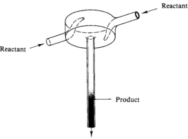
The analytical techniques so far mentioned require from a few seconds to carry out, as with optical density determinations, to minutes or hours, for chemical procedures. Many reactions are much faster than this, and a number of ingenious methods have been developed for such cases. For example, reaction times of as low as a few milliseconds can be studied with fast-mixing reactors. As illustrated in Fig. 1 4 - 5 , the separate reactant gases are jetted into a chamber so designed that mixing is rapid and complete, and the mixed gases exit into a viewing chamber.

One then determines optical density of the mixture by allowing a steady light beam to shine through the chamber and measuring its reduction in intensity.

The average lifetime of the mixture can be estimated from the inlet flow rates and the volume of the mixing chamber, and each measurement is thus for one particular time of reaction. One varies the inflow rates to vary the reaction time.

A difficulty with this procedure is in the calculation of the average lifetime and in the fact that each measurement gives only one point on the plot of amount of reaction versus time. An alternative procedure is to stop the flow of the mixed gases (such as by means of an electrically operated gate) and then to observe the progress of the reaction in the now stationary mixture in the viewing chamber.

To do this, the monitoring light beam must impinge on a light detector, such as a photomultiplier tube, whose output can go to an oscilloscope. The sweep of the oscilloscope then traces the decay of the reactants with time. Reactions involving N 0² have been much studied by this type of technique since its intense brown color makes its disappearance very easy to follow.

FIG. 14-5. Mixing cell for the study of fast reactions.

144 RATE LAWS AND REACTION MECHANISMS 557

14-4 Rate Laws and Reaction Mechanisms

Once an experimental rate law has been determined attention turns to the actual sequence of chemical steps that produces the reaction, that is, to the nature of the reaction path or mechanism. Such steps are known as elementary chemical reactions, as distinguished from the overall reaction. With two exceptions, discussed further in Sections 14-7 and 14-CN-l, we take all elementary reactions to be bimolecular, that is, to involve the reaction together of just two molecules. We proceed in this section to see how various overall rate laws can result.

A. Simple Reactions

A simple reaction is defined here as one for which the overall process and the elementary reaction are the same. The simple reactions that have been studied fall into perhaps three categories, summarized in Table 14-2. Association reactions, as the name implies, involve the combining of two molecules to give a single product. Exchange reactions are ones in which an atom or a group is transferred from one molecule to another. A very large number of such reactions have been studied; for example, many organic molecules and radicals can exchange hydrogen or halogen atoms. Decomposition reactions may be ones in which two molecules of a species combine to then break up into simpler products. These are often exchange reactions.

The experimental observation is that the mass action law, in its historic form, applies to simple reactions. That is, the rate law corresponds to the overall chemical reaction. Thus for the exchange reaction

N O + C 1 N 0² = N O C 1 + N 0⁵

A very closely related photochemical technique is that of flash photolysis.

The reactive species is now produced by a short, intense flash of light, and its decay is followed by the same monitoring light beam-oscilloscope method as before. Light flashes containing perhaps 1 0^{- 7} mole of light quanta can be made to occur within a few microseconds by triggering of the discharge of high-voltage capacitors through a gas-filled tube; xenon at about 10 Torr is often used. Many reactions involving free radicals and other reactive species have been studied by this means. Alternatively, a laser may be used to produce intense flashes of a few nanoseconds or even picoseconds duration, so that reaction times of this order of magnitude can now be studied.

These methods may be used for either gas- or solution-phase kinetics, and additional methods specially suited for solution work are described in Section 15-3.

A remaining technique that is special for gaseous mixtures is that of the shock tube. The reaction mixture is separated by means of a diaphragm from some inert gas which is at a high pressure. On rupture of the diaphragm, a shock wave passes down the reaction mixture, rapidly heating it by hundreds of degrees.

As a result of the change in temperature, reaction occurs, and it is followed, again by the monitoring light beam-oscilloscope technique. Reaction times of the order of microseconds may thus be studied.

T A B L E 14-2. Some Simple Reactions

Type Example

Association 2 N 0² N²0⁴ 2CH3 —• C²H$

Exchange N O + C 1 N 0² — NOC1 + N 0² N 0² + 0³ -> N 0³ + 0² C O + C l² — COC1 + CI Η + D² - > H D + D Η + HC1 H⁸ + CI C H³ + H² - > C H⁴ + Η C H³ + N H³ - > C H⁴ + N H² Decomposition C3H7I —> C³H^e + H I

the rate law is

Rt = - </(NO)

dt = fc(NO)(ClN0²).

B. Two-Step Mechanisms. Rules for Obtaining a Rate Law from a Mechanism A rather frequent situation is that in which a bimolecular reaction produces an intermediate which in turn reacts with itself or with one of the original reactants.

The reaction 2NO + H² N²0 + H²0 [Eq. (14-37)] is one example. The mechanism seems likely to be

2 N O = N²O^a (rapid equilibrium),

N²0² + H² ^ N²0 + H²0 (slow step).

The rules for constructing the rate law from a reaction mechanism are that, first, the mass action principle is applied to each elementary step, or to the slow step if all others are fast. This slow step determines the overall reaction rate, but it is then conventional to use the equilibrium constants and the stoichiometry of the other steps of the mechanism to express the rate law purely in terms of species that appear in the overall reaction.

The example provides an illustration of these rules. We first apply the mass action law to the slow step:

</(N,Q) dt

<*(N²0²)

dt = fc(N²0²)(H²).

However, N²0² does not appear in the overall equation (14-37), and we may eliminate it by using the equilibrium constant expression Κ = ( N²0²) / ( N O )² to get

d(N2Q)_

dt ' = fc*(NO)²(H²), (14-39) which is the observed rate law [Eq. (14-38)].

14-4 RATE LAWS AND REACTION MECHANISMS 559

Note, however, that the alternative mechanism

N O + H2 = N O · H2 (rapid equilibrium),

N O · H2 + N O ^ N20 + H20 (slow step),

where N O · H² is an association complex, equally well reproduces the experi­

mental rate law (the reader might verify this statement). Thus even in this simple situation at least two alternative paths can be thought of, both chemically reason­

able and both agreeing with the kinetic results. The similar type of reaction 2 N O + X² = 2 N O X is known, with X² = O^a, C l², or B r², and the same ambiguity of mechanism is present. One of the applications of fast reaction techniques has been to the identification of reaction intermediates so as to allow a decision to be made between alternative mechanisms. It has not yet been determined, however, whether in the cases cited the intermediate is N²0² or N O · X².

A further point is that by either mechanism the experimental rate constant is seen to be a product of a true rate constant and the equilibrium constant for the precursor reaction. This type of situation presents a very real problem in the theoretical analysis of rate data; reaction rate theories deal with elementary reactions and can easily lead to erroneous conclusions if applied to composite rate constants.

C . The Stationary-State Hypothesis

The two-step mechanism just discussed is a special case of a more general situation. It was assumed that the first step consisted of a rapid equilibrium, but the more complete analysis would be as follows:

2 N O % N20²,

N²0² + H² *X N²0 + H²0 .

We now write the sum of the mass action rate expressions for each process whereby a given species should change in concentration with time:

\ ⁼ - ^ ^{N O} > ² + ^fc-i(^N20²), (14-40)

</(N²Q²) = ^ ( N O )² - ^(Ν²0²) - fc²(N²0²)(H²), (14-41) dt

*NPL =

fc²(N²0²)(H²). (14-42)

The set of three differential equations must now be solved simultaneously. Although this can be done in the present case, the mathematics of such situations rapidly becomes intractable, and a very useful approximation is usually made so as to simplify matters. If an intermediate I, in this case N²0², is being produced and consumed in such a manner that its concentration never becomes appreciable, this means that the total reaction "traffic" is large compared to the amount of intermediate and hence that the latter rapidly attains a steady level of concentration

which then slowly drops as the reactants are consumed. The further implication is that, in this case, d(N²0²)/dt is small compared to d(NO)/dt or d(N²0)/dt; if ( N²0²) is, say, 10"³(NO), then d(N²0²)/dt should be about 10"³ d(NO)/dt, and hence 1 0^{- 3} times each of the terms of Eq. (14-41). The approximation that is therefore made is to set d(I)/dt equal to zero. This is known as the steady- or stationary-state approximation.

Application of the stationary-state approximation to the present example sets d(N²0²)/dt = 0 and allows Eq. (14-41) to be solved for ( N²0²) :

Insertion of this result into Eq. (14-42) gives

rf(N²Q) _ fc²fci(NO)²(H²)

dt *_i + A:.(H^a) * (14-44) Notice that if k_^x is large compared to A:²(H²), then Eq. (14-44) reduces to Eq. (14-39), since Κ = kjk_^t. On the other hand, at very large (H²), it should be possible to obtain the other limiting form:

rf(I^^Q) - ^ ( N O )². (14-45)

Were the alternative mechanism, involving N O · H² as intermediate, the correct one, then at large (NO), the limiting form should be

= ^ ( N O ) ( H²) . (14-46)

Investigators have attempted such studies as a means of distinguishing between the two mechanisms, but without success in that they could not reach sufficiently high pressures to observe departures from the normal rate law. However, success in this respect has been achieved in some related situations that will be discussed in Section 14-7.

D . Chain Reactions

A chain reaction is one in which some intermediate or intermediates are con­

sumed and regenerated in a cycle of reactions the net result of which is to carry forward the overall reaction. Analysis of such systems can be quite complicated, and the following example will serve to illustrate both the type of mechanism encountered and a further application of the stationary-state hypothesis.

The reaction

H2 + Br2 = 2HBr (14-47)

has been extensively studied from the time of M. Bodenstein around 1906. Unlike the situation with the seemingly analogous reaction H² + I² = 2HI, the experi­

mental rate law is very complex:

</(HBr) k^t(H²)(Br²)^

dt 1 + [^(HBr)/(Br²)]' (14-48)

14-4 RATE LAWS AND REACTION MECHANISMS 561 where k^{ has been called the inhibition constant and the term in the denominator reflects the inhibition of the reaction rate by the product HBr. The mechanism for this reaction seems now well established as the following:

B r² + Μ 2Br -f Μ (chain initiation), 2Br + Μ B r² + Μ (chain termination),

Br + H² ^ H B r + Η (chain propagation),

*3 *4

Η -f B r² HBr + Br (chain propagation).

(M is any gaseous species, and serves to supply the energy for the dissociation—

see Section 14-CN-l.) Note that the last two reactions together constitute a cycle, the net effect of which is to carry out the overall reaction [Eq. (14-47)]; this pair then constitutes the chain reaction.

The stationary-state assumption is now applied to the intermediates Η and Br:

= 0 = 2^(Br²)(M) - fc²(Br)²(M) - A:³(Br)(H²) + fc⁴(HBr)(H) + fc⁵(H)(Br²) and

(14-49)

= 0 = fc³(Br)(H²) - fc⁴(HBr)(H) - fc⁵(H)(Br²) (14-50) or

Also, addition of Eqs. (14-49) and (14-50) leads to

(Br) =

[ - ^ P f

²

=

^{K$(BTM (14-52)}

where K^lt2 is the equilibrium constant for the dissociation of Br² into atoms;

notice that (M) has cancelled out.

The rate of production of HBr is given by

= *³(Br)(H²) - fc⁴(HBr)(H) + A:⁵(H)(Br²) (14-53) and replacement of (H) and (Br) by the appropriate expressions yields

</(HBr) _ 2A:³A:^{1 1},^{/ 2 2}(H²)(Br²)^{1 / 2}

dt 1 + [A:⁴(HBr)/A:⁵(Br²)]' (14-54) which is the same as the observed rate law [Eq. (14-48)].

Many oxidation reactions proceed through a chain mechanism, and a particular example, H² + | 0² = H²0 , is discussed in Section 14-CN-4 as illustrative of systems that can lead to explosions. In addition, the thermal decomposition of many gaseous organic molecules involves free radical chains. Usually, however, thermal decomposition or pyrolysis is complicated by the presence of a large variety of products due to the various types of decomposition reactions that can occur. It has therefore been useful to initiate such decompositions photochemically;

the first step is then more apt to be a simple one, and the whole reaction sequence can be followed at a low enough temperature that intermediates and reaction products do not themselves pyrolyze.

Perhaps the most studied system of this last type is that of the photodecomposition of acetone.

Hundreds of publications have appeared o n the subject, and it must suffice here to sketch the main conclusions. Irradiation of acetone vapor with light of around 254 n m wavelength results in its fragmentation to give C H³C O , C H³, and C O :

C H³C O C H^s- > j^{c o + 2}

The following reactions then appear to be important:

2 · C H³ -> C²H^e (association),

2 · C O C H³ - > ( C H³C O )² (association),

• C H³ + · C O C H³ C H³C O C H³ (recombination),

• C H³ + · C O C H³ ->• C H⁴ + C H²= C O ( H exchange),

• C O C H³ + Μ — C O + · C H³ + Μ (decomposition),

• C H³ + · C H²C O C H³ - > C H³C H²C O C H³ (association),

• C H³ + C H³C O C H³ — C H⁴ + · C H²C O C H³ (H exchange),

• C H²C O C H³ — · C H³ + C H²= C O .

(For clarity radicals are marked with an electron dot.) The products thus include C O , C H⁴, C²H^e, C²H⁵C O C H³, and C H²= C O , with the various indicated radicals as chain carriers. N o t i c e that all but one of the elementary reactions are bimolecular. The last reaction, however, shows a unimolecular decomposition process.

14-5 Temperature Dependence of Rate Constants

The preceding material has presented the customary procedure of expressing a reaction rate in terms of a rate law, or function of concentrations of species, and the concept of reaction mechanism, whereby the mass action principle is applied to the one or more elementary reactions that are responsible for the overall process. All dependences of a reaction rate other than on concentration are thus contained in the rate constant (or constants if the rate law is a complex one). We now examine the temperature dependence of reaction rates, that is, of rate constants.

A preliminary historical review seems appropriate at this point. The mass action principle developed during the period 1850-1890, beginning with the observation by L. Wilhelmy that the rate of inversion of cane sugar was propor­

tional to the amount of unconverted sugar, the reaction being

H²0 + C^{1 2}H^{2 2}Oⁿ — C^eH^{1 2}O^e (glucose) + Q H^{1 2}O^e (fructose).

Wilhelmy integrated the first-order rate equation and, in effect, developed much of the material of Section 14-2A. The first emphasis on chemical equilibrium as the result of a dynamic balance of equal forward and reverse rates came from C. Guldberg and P. Waage in 1867, who also clearly formulated the law of mass action. Later, van't Hoff added that the equilibrium constant should then be given by Κ = kijkx). It was not until 1865, however, that the first second-order reaction was clearly defined experimentally, by Harcourt and Essen (1865, 1866, 1867), in a study of the reaction between permanganate and oxalate ions. Thus the subject of reaction kinetics evolved through the study of solution rather than

14-5 TEMPERATURE DEPENDENCE OF RATE CONSTANTS 563 gas-phase reactions, although we will see that it is for the latter that theory is best developed today.

The preceding developments set the stage for Arrhenius to observe in 1889 that rate constants showed much the same temperature dependence behavior as did equilibrium constants, namely,

d(lnk) _ constant dT ~ T²

By analogy with the second law equation, Eq. (7-29), for equilibrium constants, it was natural to write

*S°*> =

_{dT RT} ^(14-55)

2 ' ^{K D D )}

where E* represents some characteristic energy that must be added to the reactants for reaction to occur. We call is* the activation energy of the reaction.

Equation (14-55) has the usual alternative forms. Integration gives E*

In k = constant ^ = r , (14-56) so that a plot of In k versus l/T should give a straight line of slope —E*/R.

An equivalent form is

k = A e~^E*^/RT (14-57)

and integration between limits gives

- <"-

⁵⁸

>

These various forms are all known as the Arrhenius equation for rate constants;

the constant A is called the preexponential or frequency factor.

As the equations imply, reaction rates increase as temperature increases;

around 25°C, for example, a doubling of k with a 10°C rise in temperature corre­

sponds to about 12 kcal m o l e^{- 1} for E*⁹ and a quadrupling of the rate, to 24 kcal m o l e^{- 1}, and so on. The factor by which k increases over a 10°C interval is known as the temperature coefficient.

Example. E* i s 35 kcal m o l e "¹ for a certain reaction. B y what factor w o u l d k increase b e ­ tween 100°C a n d 110°C? B y Eq. (14-58),

ln(*

^M

t/*«7i)

= [(35,000)/(1.987)][(10)/(383.15)(373.15)]

= 1.23. T h e factor is thus 3.43.

The Arrhenius equation is amazingly well obeyed by systems showing a rate law of the type of Eq. (14-2). The reaction 2 H I H² + I² obeys second-order kinetics over a wide range of conditions and some of Bodenstein's data (1894-1899) are plotted in Fig. 14-6 according to the form of Eq. (14-56). The values of k are given in Table 14-3 along with those calculated from the best-fitting straight line in the Arrhenius plot. The agreement is within about 25 % over five orders of magnitude variation in k. This best straight line is given by

k^t = 9.17 χ io^{1 0}e-^{4 4}-^{4 5 0}/*^r, (14-59) where kt is in liters per mole per second.