Mőhelytanulmányok Vállalatgazdaságtan Intézet
1093 Budapest, Fıvám tér 8.
(+36 1) 482-5566, Fax: 482-5567
www.uni-corvinus.hu/vallgazd
A Dynamic Input-Output Model with Renewable Resources
Imre Dobos Péter Tallos
137. sz. M ő helytanulmány HU ISSN 1786-3031
2011. április
Budapesti Corvinus Egyetem Vállalatgazdaságtan Intézet
F ı vám tér 8.
H-1093 Budapest
A Dynamic Input-Output Model with Renewable Resources
Imre Dobos
1Péter Tallos
21 Corvinus University of Budapest, Institute of Business Economics, H-1093 Budapest, Fıvám tér 8., Hungary, imre.dobos@uni-corvinus.hu
2Corvinus University of Budapest, Department of Mathematics, H-1093 Budapest, Fıvám tér 13-15., Hungary, tallos@uni-corvinus.hu
Absztrakt.
A dolgozat a dinamikus input-output modell egy általánosítását tárgyalja. A sztenderd dinamikus Leontief-modellt terjesztjük ki arra az esetre, amikor a megújuló er ı források egyenleteit is a modellhez csatoljuk. A megújuló er ı források készletei növekednek a regenerációs rátával, amit csökkent a felhasználás üteme. Ebben a dolgozatban az új modell irányíthatóságát vizsgáljuk, a fogyasztási rátát tekintve irányítási változónak. Az egyensúlyi arányos pályát vizsgálva arra keresünk választ, hogy milyen növekedési ütemet képes elérni a gazdaság anélkül, hogy kimerítené a megújuló er ı forrásokat. A megoldásban az irányításelmélet és a klasszikus lineáris algebra eredményeit használjuk fel.
Kulcsszavak: Dinamikus rendszerek, Sajátérték feladat, Irányításelmélet, Környezeti menedzsment
Abstract.
The paper studies a generalisation of the dynamic Leontief input-output model. The standard dynamic Leontief model will be extended with the balance equation of renewable resources.
The renewable stocks will increase regenerating and decrease exploiting primary natural resources. In this study the controllability of this extended model is examined by taking the consumption as the control parameter. Assuming balanced growth for both consumption and production, we investigate the exhaustion of renewable resources in dependence on the balanced growth rate and on the rate of natural regeneration. In doing so, classic results from control theory and on eigenvalue problems in linear algebra are applied.
Keywords: Dynamical Systems, Eigenvalue Problem, Control Theory, Environmental Management
A Dynamic Input-Output Model with Renewable Resources
Imre Dobos
∗and Peter Tallos
†Abstract
The paper studies a generalisation of the dynamic Leontief input- output model. The standard dynamic Leontief model will be extended with the balance equation of renewable resources. The renewable stocks will increase regenerating and decrease exploiting primary natural re- sources. In this study the controllability of this extended model is ex- amined by taking the consumption as the control parameter. Assuming balanced growth for both consumption and production, we investigate the exhaustion of renewable resources in dependence on the balanced growth rate and on the rate of natural regeneration. In doing so, classic results from control theory and on eigenvalue problems in linear algebra are ap- plied.
Keywords: Dynamical Systems, Eigenvalue Problem, Control The- ory, Environmental Management
1 Introduction
Solving environmental problems such as the exhaustion of natural resources urges a thorough analysis of the interaction between the development of the economy and the natural environment. In this paper we present an environ- mental impact study focusing on the interdependence of the economic activities and the associated flow of renewable resources. Despite its known simplifica- tions, input-output analysis is a useful instrument to study strategic directions of economic development, extending dynamic intersectoral links also to the in- teraction between the sectors of economy and the natural environment. Such an analysis is important for the development of state regulation programs, which are an integral part of environmental-economic policy for any developed market system (Field, [8]).
∗Institute of Business Economics, Corvinus University of Budapest, Hungary, imre.dobos@uni-corvinus.hu, (Corresponding author)
†Department of Mathematics, Corvinus University of Budapest, Hungary
In the economic literature renewable resources are often examined. The first known paper on this field was published by Hotelling in year 1931. This first applications analysis investigate the fishery processes (Clark, [3]). These types of model use logistic differential equation to describe the motion of the prob- lem. The models are then characterized by profit function to maximize the present value. A second direction analyzes a growth model in general equilib- rium context. In these models the discounted utility function of the economy is maximized (Ayong Le Kama, [2], Wirl, [14]). Similar models are investigated by Elíasson and Turnovsky [7] who look for macroeconomic equilibrium and a balanced growth. The use of renewable resources raises the question of sustain- ability of the resource utilization policy (Valente, [13], Li and Löfgren, [11]). All of these models apply continuous time economic models.
In this study, we consider the well-known dynamic Leontief input-output model augmented with the balance equation of regenerative natural resources (Leontief, [10]). One of the questions arising in this ecological input-output model is whether this dynamic model is controllable if consumption is taken as the control parameter? In other words, can the use of the natural resources be influenced by controlling the consumption in the economy? The other question we intend to answer is how the rate of regeneration of a renewable resource influences growth rate for both consumption and production, if an environmental regulation agency does not want to fully exhaust a renewable resource.
This paper is a natural extension of our former results for renewable resources in the case of a singular matrix of capital coefficients (see Dobos and Floriska [5], [6]).
For our investigations we use classical results from control theory and eigen- value problems in linear algebra. The next section presents the basic equation system of the augmented dynamic Leontief system. The following sections exam- ine the controllability and the balanced growth path of the system respectively.
Finally, we illustrate our results for a simple numerical example.
2 The Dynamic Leontief Model
Our model is based on the equations of the dynamic multi-sector input-output model well known in the literature (Leontief, [10]). We extend this model with the balance equation of renewable resources in order to analyse the linkage between the economy and the environment.
Suppose that there are n economic industries, each industry producing a single commodity andmprimary resources used by the sectors of productions.
(Each industry may use more resources and let us suppose thatm < n). The input-output balance of the entire economy can be described by the equations for goods and resources. The equation for goods describes the balance between the total output of goods and the sum of total inputs of goods and the consumed goods.
Let us consider
x(t) =Ax(t) +Bx(t) +˙ c(t) (1) wherex(t)is the nonnegative n-dimensional vector of gross industrial outputs in year t; c(t) is the n-dimensional vector of final consumption demands for commodities in yeart; Ais then×nmatrix of input coefficients, showing the input of goods that are required to produce one unit of a product; and B is the n×n matrix of capital coefficients, where the element bij is the capital requirement of goodinecessary for the increase of one unit of output in sector j. It is assumed that the matrix of capital coefficients is singular, i.e. it is not invertible.
The equation for resources describes the relation between the stocks of renew- able resources in two subsequent years, taking the regeneration and exploitation in a given year into account.
Now consider
N˙(t) =< g > N(t)−Ex(t) (2) whereN(t)is the nonnegative m-dimensional vector of renewable resources in yeart,g is them-dimensional vector of rates of natural regeneration of natural resources and < g > is an m-dimensional diagonal matrix, with the rates of regeneration of the resources in the diagonal. E is the m×nmatrix of input coefficients of resources, where the elementEij is the requirement of resourcei to produce one unit of output in sectorj.
Throughout this paper we assume that:
• the matricesA,B andE are nonnegative,
• the matrixAis productive and its Leontief inverse(In−A)−1 is nonneg- ative, whereIn is then×nidentity matrix,
• B is singular,
• c(t)is a nonnegative vector.
The two equations above can be written in explicit vector form:
B 0 0 Im
· x(t)˙
N˙(t)
=
In−A 0
−E < g >
· x(t)
N(t)
− In
0
·c(t) (3) and because of the singularity of the2×2 matrix on the right-hand side, con- trollability of system (3) cannot be analyzed by using the classical Kalman’s condition (see Aoki, [1]). We must solve this system explicitely to express the solution of the linear diffential equation system. This system is solvable be- cause matrices of system (3) build regular matrix pencils (Gantmacher, [9]).
The regularity of the matrix pencils can be proven easily:
λ
B 0 0 Im
−
In−A 0
−E < g >
=
λB−(In−A) 0 E λIm−< g >
Ifλ= 0in the last expression then the matrix on the right-hand side is invertible, and
In−A 0
−E < g >
−1
=
(In−A)−1 0
< g >−1E(In−A)−1 < g >−1
This means that model (3) is solvable and there exists an explicit solution (Gant- macher, [9]).
3 Controllability of the Model
The controllability of a system means that the system can be steered from any given initial state to any other state in a finite time period by means of a suitable choice of the control function (Aoki [1]). Applying Kalman’s theorem (Aoki [1]) we get that system (3) is controllable if and only if the rank condition is satisfied.
Note that[B, AB, . . . , Am+n−1B]is an(n+m)×(n+m)matrix.
Theorem 1 The system (3) is controllable if and only ifrank E=m.
Proof. Consider the time interval[0, T]and a solutionxto (1) withx(0) =x0
andx(T) =xT. Consider them×mmatrix< g >and denote byΦthe matrix solution to the homogeneous linear system
N˙(t) =< g > N(t) (4) LetE be a realm×nmatrix with rankmand consider the following subset of allRn-valued continuously differentiable functions on the interval [0, T]
C0,T ={x∈C1[0, T] : x(0) =x0, x(T) =xT}
Define the linear mappingΛ :C1→Rm by Λx=
Z T 0
Φ(t)−1Ex(t)dt
Under the above conditions the system (3) is controllable, i.e.
Λ(C0,T) =Rm if and only if the matrixE is of full rank.
The necessity of the condition is obvious. To prove the sufficiency, letv∈Rm be given arbitrarily. We have to find anx∈C0,T with
v= Λx= Z T
0
Φ(t)−1Ex(t)dt
Introduce the notations y0 = Ex0 and yT = ExT. Clearly, if we can find a continuously differentiable function y : [0, T] → Rm with y(0) = y0 and y(T) =yT further with
v= Z T
0
y(t)dt (5)
then the function defined by
Ex(t) = Φ(t)y(t) (6)
fulfills the criteria of the theorem.
In order to find anywith this property, pick any continuously differentiable functionyˆon[0, T]withy(0) =ˆ y0 andy(T) =ˆ yT. Suppose
Z T 0
ˆ
y(t)dt=w∈Rm
Letαandβbe undefined real parameters and consider the family of continuously differentiable functions
yα,β(t) = ˆy(t) +αt(T−t)v+βt(T−t)w
for everytin[0, T]. It can be verified easily thatyα,β still satisfies the boundary conditions, i.e. yα,β(0) =y0andyα,β(T) =yT for every realαandβ. Moreover, a straightforward calculation shows that for appropriate values of αandβ we have
Z T 0
yα,β(t)dt=v
For thoseαandβ introduce
y(t) =yα,β(t) = ˆy(t) +αt(T−t)v+βt(T−t)w and consider the equation
Ex(t) = Φ(t)y(t)
on the interval[0, T]. On the one hand the vector spaceRmcan be given as the direct sum of the orthogonal subspaces
Rm= kerE⊕imE∗
whereE∗ stands for the adjoint of the matrix E, on the other handE creates an isomorphism between them-dimensional spacesRm and imE∗. Therefore, for any y there exists a continuously differentiable function x on [0, T] with x(0) =x0andx(T) =xT that is a solution to (3).
Remark. The controllability of system (3) could also be proved by the clas- sical matrix conditions for singular systems (cf. Dai, [4]). The reason why we have chosen this explicit approach is to demonstrate the special structure of
the economic-ecological system. The linear system (3) consists of two types of differential equations. The first (1) points out the economic system, while equations (2) represent the ecological system. In other words, the economic model influences the ecological system. Our proof relies on this phenomenon and captures some insight into the structure of the economic-ecological nature of the model. Here we briefly sketch how to exploit the matrix conditions by Dai, [4]. The condition possesses the form
rank
s·
B 0 0 Im
−
In−A 0
−E hgi
; −In
0
=n+m
for all scalars s∈ R. Verifying this rank condition assume that there exists a vectorv= [v1, v2]such that
[v1, v2]·
s·B−(In−A) 0 E s·Im− hgi
; −In
0
= [0,0]
i.e. the rows of the matrix are dependent. By carrying out the multiplications we get the following system
v1·[s·B−(In−A)] +v2·E = 0 v2(s·Im− hgi) = 0
−v1 = 0
Substituting the third equation into the first, we obtain thatv1= 0andv2= 0 which proves the condition.
For a policy implication of this result, suppose that the government or a reg- ulatory organization wants to regulate the stocks of renewable natural resources.
For example, in the context of sustainable development to save the stocks, this can be done by controlling the level of the consumption rate. The slow-down of the exploitation of renewable resources will increase the possibilities of the next generations to get hold of natural resources. The assumption on the linear independence of the row vectors of input coefficients of resources can be held because of the non-substitutability of various natural resources.
4 The examination of resources along the Bal- anced Growth Path
The linear system in (3) is controllable in the usual mathematical sense. How- ever, economics also requires the nonnegativity of the control and the state variables. In this section we will examine this issue for the case of a balanced growth path for both production and consumption. Fixing a given control (that is, for a given consumption), we examine the trajectories of system (1) and the effect of a balanced path on the use of the renewable environmental resources.
We study the balanced growth solution of the system (1) under the assump- tion that both production and consumption increase at the same given growth rateα≥0. That is,x(t) =x0eαt and c(t) =c0eαt. Substituting these expres- sions in equation (1), yields that the following equality must hold:
(In−A−αB)x0=c0. (7)
This equation indicates that the output configurationx0 corresponding to the balanced growth path, depends on bothαandc0. Define the marginal growth rate α0 such that the Frobenius root (or dominant eigenvalue) of the matrix A+α0B equals one (see Schoonbeek [12]). The solution is given by
x0(α) = (In−A−αB)−1c0 (8) Next, we investigate the evolution of the stocks of renewable resources corre- sponding to the balanced growth path of system (3). Substitutingx(t) =x0eαt in equation (2) and applying a simple procedure gives the following result for the stocks of resources:
N(t) =e<g>tN0− e<g>t−eαImt
·(< g >−αIm)−1Ex0(α) (9) Theorem 2 For every indexiandα≤gi, the stock of resourcesNi(t)remains nonnegative over the time horizont∈[0,+∞).
In addition, for every indexiand for every fixedt∈[0,+∞)the stockNi(t) is monotone decreasing
(i) with respect toαon the interval0≤α < α0 and (ii) with respect to any nonnegative consumption vector c0.
Proof. The first property can be verified easily by equation (9). The second property follows from examining the appropriate derivatives.
In economic terms, this theorem states that renewable resources will be not fully exhausted if the rate of growth is lower than the minimal rate of regener- ation. In other case, i.e. growth rate is greater than the regeneration rate, the renewable resources can be considered, as a non-renewable resource. The envi- ronmental protection agencies must stimulate such an economic growth as not greater than the regeneration rate of natural regenerative resources. In a bal- anced growth economy the government and/or regulatory organisation have two economic indicators to control the exploitation of renewable natural resources:
a reasonable growth rate, or proportion of the consumption level. The regu- lation of the growth rate has a direct effect on the exploitation of the natural resources. A reduction of the growth rate will decrease the exploitation of the resource levels. The influence of the consumption level is twofold: a proportional decrease of final demand for all sectors reduces the resource exploitation. In a
non-proportional case, however, restricting the final demand in sectors with a high use of natural resources can reserve resources for sectors with lower use of natural resources. In this sense there is a potential trade-off between balanced growth rate and balanced consumption level. The consumption level can be increased with a lower growth rate to hold the available natural resources for future generations.
5 A Numerical Example
In order to illustrate the functioning of the proposed model, we take a simple case by aggregating the investigated economic system into three major sectors, assuming that each producing sector uses two types of resources. We set the parameters of the matrices of input coefficients, capital coefficients and resource coefficients as follows.
A=
0.1 0.3 0.2 0.5 0.2 0.4 0.2 0.4 0.5
B=
0.01 0.03 0.02 0.05 0.02 0.04
0 0 0
and
E=
0.6 0.2 0.1 0.4 0.5 0.3
g= 0.2
0.3
Using the results of Theorem 2, the marginal growth rate of the model is α0 = 0.792, but the minimal rate of regeneration is min1≤i≤2gi = 0.2. This means that a rational growth rate must be lower than this threshold. Let us assume next that the vectors c0 of initial consumption levels and N0 with the initial stock of exhaustible resources are
c0=
1 3 2
and N0=
10,000 15,000
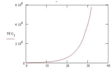
Let us now investigate two cases. In the first case we assume that the growth rate is equal to 0.28. For this growth rate the first renewable resource is actually a non-renewable resource, because the growth rate is greater than the rate of natural regeneration, α > g1. After some calculations it can be seen that the first resource lasts 34 years. Figures 1 and 2 show these resources. The second natural resource is a renewable resource, because the growth rate is smaller than the rate of natural regeneration, i.e. α < g2.
In the next example we assume that the growth rate is 0.1, i.e. α = 0.1.
In this example the growth rate is smaller than both of the rate of natural regeneration, i.e. α < g1< g2, so for this economy the renewable resources will not be totally exhausted under this growth rate.
Figure 1: The stock level of the first natural resource forα= 0.28
Figure 2: The stock level of the second natural resource forα= 0.28
Figure 3: The stock level of the first natural resource forα= 0.1
Figure 4: The stock level of the second natural resource for α= 0.1
6 Conclusions and Further Research
In this paper we have investigated a generalised dynamic Leontief model. The basic model was extended with regenerative resources. It was shown that this augmented model is controllable if the input matrix of resources has a full rank. In the second part of the paper we have examined the effect of the balanced growth path on the resource exploitation. It was shown that the stock of renewable resources lasts if the regeneration rates of natural resources are higher than the growth rate.
A topic for further research would be the effect of the balanced growth path on the quality of the renewable environmental resources. The question is how the use of the environmental resources (emission) will influence this balanced path if the emission level is limited by a legal environmental standard. A second possibility would be to extend the present model with the recycling of reusable materials. In this case the coefficients of the input matrix of resources will be reduced and the environmental resources will last longer. Such an investigation may be relevant in the context of sustainable development. Note that these investigations (as well as the model that we have used in this paper) ignore the influence of prices on the growth path. Considering the dual problem could shed some light on the issue of economic efficiency of production. Developing a new price system could control the production in an environmental-conscious way.
References
[1] Aoki, M., Optimal Control and Systems Theory in Dynamic Economic Analysis, North-Holland, New York, Oxford, Amsterdam, 1976.
[2] Ayong Le Kama, A. D., Sustainable growth, renewable resources and pollution,J. Economic Dynamics & Control, 25 (2001), pp. 1911–1918.
[3] Clark, V. W., Mathematical models in the economics of renewable re- sources,SIAM Review, 21 (1979), pp. 81–99.
[4] Dai, L., Singular Control Systems, Springer-Verlag, New York, Berlin, 1989.
[5] Dobos I., Floriska, A., A dynamic Leontief model with non-renewable resources,Economic Systems Research, 17 (2005), pp. 319–328.
[6] Dobos I., Floriska, A., The resource conservation effect of recycling in a dynamic Leontief model,Int. J. Production Economics, 108 (2007), pp.
334–340.
[7] Eliasson, L., Turnovsky, S. J., Renewable resources in an endoge- nously growin economy: balanced growth and transitional dynamics, J.
Environmental Economics and Management, 48 (2004), pp. 1018–1049.
[8] Field, B. C.,Environmental Economics: An Introduction, McGraw-Hill, New york, 1997.
[9] Gantmacher, F. R.,Theory of Matrices, Chelsea, New York, 1959.
[10] Leontief, W. W., Input-Output Economics, Oxford Univesity Press, Oxford, New York, 1986.
[11] Li, C.-Z., Löfgren, K.-L., Renewable resources and economic sustain- ability: a dynamic analysis with heterogeneous time preferences,J. Envi- ronmental Economics and Management, 40 (2000), pp. 236–250.
[12] Schoonbeek, L., The Size of the Balanced Growth Rate in the Dynamic Leontief Model,Economic Systems Research, 2 (1990), pp. 345–349.
[13] Valente, S., Sustainable development, renewable resources and techno- logical progress, Environmental & Resources Economics, 30 (2005), pp.
115–125.
[14] Wirl, F., Sustainable growth, renewable resources and pollution: thresh- olds and cycles,J. Economic Dynamics & Control, 28 (2001), pp. 1149–
1157.