Cost minimization of compressed I-section columns with different design rules

(1)

1 1 INTRODUCTION

Stability is one of the most important problems in the design of welded metal structures since the instability causes in many cases failure or collapse of the structures.

The normal stresses and overall stability are calculated for pinned columns. The dimensions of the I-columns are optimized by using constraints on overall stability, local buckling of webs and flanges. The calculations are made for different loadings, column length and steel grades.

The yield stress varies between 235 and 690 MPa.

2 DESIGN RULES ACCORDING TO DIFFERENT STANDARDS The general overall buckling rule is the following

N  Af_y/ _M₁ (1) Buckling parameter  is calculated according to Eurocode 3 (2005) on the following way

   

   

  

  

2 2

2 2 2

1 (2)

^ ^^{0 5 1}^.



^^^b ^^²



and ^^b ^^{ }



^^{0 2}^.



(3)     / _E; _E  E/ f_y (4) It should be mentioned that the EC3 formula is too complicated for design (non-computerized optimization) purposes. There exist other column curves used in other countries which can be applied instead of EC3 curves.

The Japan Railroad Association (JRA) (2012) curve is described by the following formulae 1 for 0 2.

Cost minimization of compressed I-section columns with different design rules

K. Jármai, M. Petrik

University of Miskolc, Miskolc, Hungary

ABSTRACT: The aim of the present study is to show the minimum cost design procedure for welded steel I-section columns loaded by compression force. The overall stability is calculated for pinned columns. The dimensions of the I-columns are optimized by using constraints on overall stability, local buckling of webs and flanges. The different design rules and standards are used. The cost calculation includes the material, welding, cutting and painting costs. The calculations are made for different loadings, column length and steel grades. The optimization is made using the Generalized Reduced Gradient (GRG2) method in the Excel Solver. Cost calculations and comparisons show the most economic structure.

(2)

2

 1109. 0 545.  for 0 2.   1 (5) ^ ^¹^/



^{0 773}^. ^^²



for 1

The curve of the American Petroleum Institute (API) (2004) is defined by

 1 0 25. ² for 0  141. (6)  1/² for 141.

The curve of the American Institute of Steel Construction (AISC) (2013) mainly for round tubes is given by

  1 0 091. 0 22. ² for  141. (7)  0 015. 0 834. /² for 141.

2.1 Constraints

Constraint of overall buckling is according to Eq.(1). The buckling parameters are in Eqs. (2-7).

Constraint on local buckling of web for the I-column

;

t h

w 

 1 or t_w h (8)

where

fy

;

/ 42 235

1    (9) Constraint for local buckling of compressed upper flange of I-column



 ²⁸ 1

 tf

b , or t_f b (10) 2.2 Objective function

The objective function to be minimized selected in this study can be the cost of the I-column.

In this case we consider welding, cutting and painting costs.

3. THE COST CALCULATION 3.1 The cost of materials

K_M k_MV, (11) For steel the specific material cost can be kM=1.0-1.3 $/kg depending on the thickness.

KM [kg] is the fabrication cost, kM [$/kg] is the corresponding material cost factor, V [mm³] is the volume of the structure, is the density of the material. For steel it is 7.85x10^-6 kg/mm³. 3.2 The fabrication cost in general

Kf = kf



i

Ti, (12)

where Kf [$] is the fabrication cost, kf [$/min] is the corresponding fabrication cost factor, Ti [min] are production times. It is assumed that the value of kf is constant for a given manufac- turer.

3.3 Fabrication times for welding

The times of preparation, assembly and tacking can be calculated with an approximation formula as follows

T_w₁C₁_dw V , (13) where C1 is a parameter depending on the welding technology (usually equal to 1), dw is a difficulty factor,  is the number of structural elements to be assembled. The difficulty factor expresses the complexity of the structure. Difficulty factor values depend on the kind of struc-

(3)

3

ture (planar, spatial), the kind of members (flat, tubular). The range of values proposed is between 1-4 (Farkas & Jármai 2013).

Real welding time can be calculated in the following way

_wi

i wi i

w C a L

T 2^ 2 ² , (14) where awi is weld size, Lwi is weld length, C2i is constant for different welding technologies.

C2 contains not only the differences between welding technologies, but the time differences between positional (vertical, overhead) and normal welding in downhand position as well. The equations for different welding technologies can be found in the Farkas, Jármai (2013).

There are some additional fabrication actions to be considered such as changing the elec- trode, deslagging and chipping. The approximation of this time is as follows

Tw₃^0.3C₂iawi²Lwi. (15) It is proportional to Tw2. It is approximately the 30% of it. The two time elements are as follows:

^T^w²^^T^w³^¹^.³



^C²ⁱ^a^wiⁿ^L^wi. (16) The welding time for ½ V, V, K and X weldings are given for the different technologies SMAW = Shielded Metal Arc Welding, SMAW HR = Shielded Metal Arc Welding High Recovery, GMAW-CO2 = Gas Metal Arc Welding with CO2, GMAW-Mix = Gas Metal Arc Welding with Mixed Gas, FCAW = Flux Cored Arc Welding, FCAW-MC = Metal Cored Arc Welding, SSFCAW (ISW) = Self Shielded Flux Cored Arc Welding, SAW = Submerged Arc Welding, GTAW = Gas Tungsten Arc Welding

3.4 Fabrication times for cutting

The cutting and edge grinding can be made by different technologies, like Acetylene, Stabilized gasmix and Propane with normal and high speed (Farkas & Jármai 2015).

The cutting cost function can be formulated using in the function of the thickness (t [mm]) and cutting length (Lc [mm]). Parameters are given in (Farkas & Jármai 2015):

^



i

ci n i CPi

CP C t L

T , (17) where ti the thickness in [mm], Lci is the cutting length in [mm]. The value of n comes from curve fitting calculations.

3.5 Fabrication times for painting

The painting means making the ground- and the topcoat. The painting time can be given in the function of the surface area (As [mm²]) as follows:

T_CP _dp(a_gc a_tc)A_s, (18) where agc = 3x10^-6 min/mm² , atc = 4.15x10^-6 min/mm², dp is a difficulty factor, dp=1,2 or 3 for horizontal, vertical or overhead painting.

3.6 Design data

Compression force N = 20-150 [kN], Column length L = 2-10 [m],

Yield stress fy = 235, 355, 460, 690 [MPa].

Design rules: EC3=Eurocode 3, AISC=American Institute for Steel Construction, API=American Petroleum Institute, JRA=Japan Road Association.

The unknowns are the four sizes of the cross section h, tw, b, tf .

4 OPTIMUM RESULTS, COMPARISONS OF THE WELDED I-COLUMN

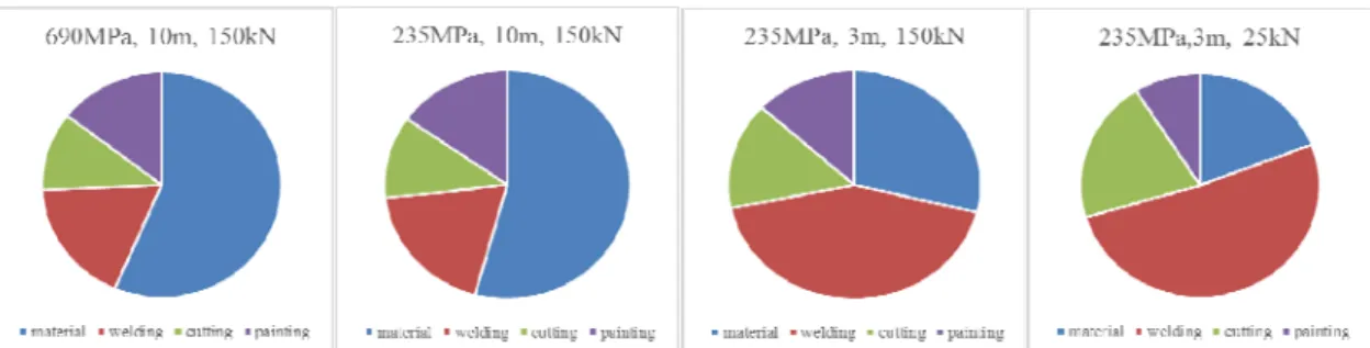
Some cost distribution can be seen on Figure 1 for the welded I-beam, when the steel grade, the length or the compression force have changed. It shows, that the material cost is dominant for long columns, the welding, cutting and painting costs are in the same range. For short columns and smaller force, the welding cost is more dominant.

(4)

4

Figure 1. Cost distribution of the welded I-beam, when the steel grade, the length or the compression force have changed

When one calculates the differences in the cost [$] in the function of the length and design rules, when the compression force is N=85 kN. The value is calculated considering the cross sections for the largest and smallest steel grade and how much percent is the difference, when the compression force is given to be 85 kN (AS690-AS235)x100%. Figure 2 shows the differences for the four design rules. The AISC has the smallest difference and the JRA has the largest.

Figure 2. The differences in the costs [$] in the function of the length and design rules, when the compression force is N=85 kN

CONCUSIONS

In the optimization process the height, the width and the thickness of the web and flanges have been optimized for the welded I-beams. The objective function to be minimized was the cost of the column, the constraints were the overall column buckling and local buckling of the web and flanges. The calculations show, that for a predesign the optimization is applicable and very use- ful. Using different standards and design rules the optimum sizes and cross sections are different. The JRA and EC3 look more conservative, the API is more liberal and the AISC is between them.

REFERENCES

American Institute of Steel Construction (2013), AISC, Design Guide 28: Stability Design of Steel Build- ings.

American Petroleum Institute (2004), API Bulletin 2V, Design of Flat Plate Structures, Third Edition.

Eurocode 3. (2005) Part 1.1. Design of steel structures. General rules and rules for buildings. European Committee for Standardization. Brussels.

Farkas, J., Jármai, K. (2013), Optimum design of steel structures. Springer Verlag, Berlin, Heidelberg Japan Road Association (2012), JRA, Specifications for Highway Bridges, Part I_V.