VALIDATION OF HEAT SOURCE MODEL FOR METAL ACTIVE GAS WELDING

VALIDATION OF HEAT SOURCE MODEL FOR METAL ACTIVE GAS WELDING

D. KOLLÁR* and B. KÖVESDI*

*Budapest University of Technology and Economics (Department of Structural Engineering, H-1111, Budapest, Hungary, 0000-0002-0048-3327, kollar.denes@epito.bme.hu)

DOI 10.3217/978-3-85125-615-4-05

ABSTRACT

The most sufficient welding parameters and settings of manufacturing technologies are currently mainly determined by experiments for standardised production in the practice. It is a time-consuming method, while there is a large amount of waste during the ’trial and error’ process of distinct welding technologies.

Virtual fabrication and virtual testing of weldments using finite element method provide a sustainable solution for advanced applications. Calibration and validation of heat source models using finite element analysis is a crucial task, because theoretically the calibration has to be done for all the individual cases related to different welding processes and welding variables. Nevertheless, it can reduce the need of on- site experiments and waste during fabrication. A comprehensive literature review has been carried out focusing on the introduction of different heat source models. The aim of the current research is to develop a common calibration process for a wide range of heat source model parameters to ensure general applicability for a typical joint of a weldment. A systematic research program is carried out on small scale specimens using different welding input parameters. The experimental research program contains temperature measurements during welding, macrographs and deformation measurements after welding.

In addition, a numerical study using uncoupled transient thermo-mechanical analysis, including sensitivity analyses and parametric studies focusing on fusion zone size, residual stresses and distortions, is performed. Based on the large number of experimental data, thermal efficiency and heat source model parameters are calibrated and verified. As a generalization, a validated heat source model is developed for a metal active gas welding power source. The developed validation process can have significant role in case of robotic welding, where welding trajectory, heat input, travel speed and quality can be controlled precisely.

Keywords: welding simulation, heat source model, calibration, validation, metal active gas welding

PROBLEM STATEMENT

There is a remarkable industrial demand on speeding up and improving manufacturing processes. Lindgren [1] revealed that welding technologies are generally developed by performing experiments and tests on prototypes, while computational methods are still rarely used in the development process. It is a substantial expectation that simulations will complement experiments using the ‘trial and error’ process for obtaining Welding Procedure Specifications (WPS) as a final result. Namely, both residual stresses and deformations are evaluated in the design phase to optimize welded structures. However,

nowadays deformations are usually in focus whereas residual stresses are of interest in subsequent phases.

In most of the cases it is time efficient and economical to use Computer-aided Engineering (CAE) opportunities rather than determining optimal parameters experimentally. Developing a sustainable virtual manufacturing process is an innovative way to reduce waste in workshops and specify optimal conditions depending on the requirements. Goldak and Akhlaghi [2] denoted that in the automotive industry the number of prototypes has been reduced from a dozen to one or two applying CAE sources as powerful, robust and efficient tools. The general aim of Computational Welding Mechanics (CWM) is to set up reasonably precise methods and models that are capable of controlling and designing welding technologies whilst ensuring suitable performance [3]. Obviously, it is an overall aim to perform numerical simulations faster and easier than to carry out welding experiments, especially when dealing with large welded structures [4]. The welding simulation procedure can be implemented in full-scale modelling frameworks describing the entire manufacturing process including steel rolling, cold forming, thermal cutting, machining, etc. [5]. An additional tremendous advantage of CWM is comparing different variants in the design phase, while performing subsequent analyses on virtual specimens, such as buckling [6-8] or fatigue analysis, is also a potential.

The determination of residual stresses and deformations are highly recommended for manufacturers as well as for designers. In case of steel structures there are often assembly difficulties and resistance problems due to large weld sizes, high heat inputs or poor clamping conditions during fabrication. These effects can result in large deformations and residual stresses, which can reduce the resistance of steel structural elements. Most of the standards, such as EN 1993-1-5:2005 [9], give only approximations for the initial (equivalent) geometrical imperfections. Therefore, it is an important task to take these effects into account as accurately as possible. Several years ago it was almost impossible to simulate the welding of large and complex structures because of hardware requirements and long computational time. Nowadays, due to the improvement of computational background it is feasible to examine large-scale welded joints and structures in an adequately accurate way, but it has to be declared that computations still have boundaries.

The aim of the current research is to develop a common calibration process for a wide range of welding variables and heat source model parameters to ensure general applicability for a typical T-joint of a weldment. A systematic research program is carried out on small scale specimens using different welding input parameters. The experimental research program contains temperature measurements during welding, macrographs and deformation measurements after welding. In addition, a numerical study using transient thermo-mechanical analysis, including sensitivity analyses and parametric studies focusing on fusion zone size, residual stresses and distortions, is performed. Based on the large number of experimental data, thermal efficiency and heat source model parameters are calibrated and verified. As a generalization, a welding process model is developed for a metal active gas welding power source. The developed validation process can have significant role in case of robotic welding, where welding trajectory, heat input, travel speed and quality can be controlled precisely.

LITERATURE REVIEW

Experiments and measurements are intended to assist in getting acquainted with heat sources. There is a fundamental need for better understanding the influence of certain parameters and more precise approaches to predict the realistic behaviour. Mathematical models are used to enhance the knowledge of heat sources taking distinct effects into account. For instance, mathematical models can include ‘the energy equation, surface tension of the weld pool surface, hydrostatic forces, Lorentz and Marangoni forces in the weld pool, pressure and shear forces from the arc or plasma, and droplet transfer to the weld pool’ according to Goldak and Akhlaghi [2]. Generally, the aim is to model the welding heat source as accurate as it is necessary depending on one’s purpose. Naturally, the level of negligence is related to the analysis aspects. Therefore, Goldak and Akhlaghi classified heat source models into five categories of First to Fifth Generation Weld Heat Source Models. The fifth class is the newest and most complex. The older ones are considered as sub-classes of each newer generation as latter generations include the attributes of former models. Table 1 sums up the pros, cons, applicability and the need for calibration of each weld heat source model generation. The following subsections introduce the history and the most important features of each heat source modelling level. The introduction focuses on the Second Generation Weld Heat Source Models as these are relevant for the presented finite element calculations; however, the subsequent generation models are presented briefly as well. Heat source models can be generalized for welding processes in a parameter range. According to Lindgren [3], welding process models are coupling the physics of the problem, the power density distribution in the weld pool and welding process parameters.

Sudnik et al. [10-11] set up such a model earlier for laser beam welding taking energy transport, vapour pressure and capillary pressure into account. Welding process models have much importance as experiments can be combined or fully replaced by calibrated heat source models in the region of interest [12].

First generation heat sources comprehend point, line and plane heat source models. Point heat source models are designated to model arc welding. Line heat source models can be used for full penetration welds, e.g., electron beam welding or laser beam welding.

Generally, plane heat source models are effective to simulate welding with sheet electrodes.

The temperature can be predicted in any point in the specimen utilizing these heat source models. The development of instantaneous point heat source models for two- and three- dimensional heat flow, solving the heat flow differential equation for quasi-stationary state, is credited to Rosenthal [13] and Rykalin [14]. Rosenthal made a few assumptions such as (i) the energy input from the heat source is uniform and moves with a constant velocity along a trajectory, (ii) all the energy is deposited into the weld at a single point, (iii) thermal properties are temperature-independent, (iv) heat flow is governed by conduction, meanwhile radiation and convection are ignored, in addition (v) latent heats due to phase transformations and fusion/solidification is neglected. Analytical approaches are effective for instance in determining the approximate size of the heat-affected zone or fusion zone, thermal gradients, phase proportions and hardness. Heat source models of Rosenthal and Rykalin have been widely used for modelling infinite or semi-infinite bodies. The temperature field far from the weld could be determined with acceptable accuracy, but the accuracy of these approaches may decrease severely in the fusion zone and the heat-affected zone. On the other hand, for welded structures with complex welding trajectories quasi-

stationary state may not even exist according to Goldak et al. [15], thus, the utilization of First Generation Weld Heat Source Models is restricted.

Table 1 Pros, cons, applicability and the need for calibration of weld heat source model generations (WHSMG).

WHSMG Pros Cons Applicability/Calibration

First analytical solution low computational cost

distribution of energy  constant material properties phase transformations  radiation and convection  simple weldment geometry straight weld path

discontinuities in geometry  constant travel speed quasi-steady state heat transfer

approximates temperature for finite, infinite or semi- infinite bodies without discontinuities and nonlinearities;

supports welding control systems and optimizing welding variables;

calibration is not really possible

Second

distribution of energy nonlinear material properties

phase transformations radiation and convection complex weld path complex weldment geometry

discontinuities in geometry varying travel speed unsteady state heat transfer

moderate computational cost

fluid flow

complex weld pool shapes

/

FDM* or FEM*:

nonlinearities;

realistic temperature fields outside of the weld pool;

complex weld pool shapes:

prescribed temperature model/combination of surface and/or volumetric heat sources;

calibration is needed

Third

Stefan problem Cauchy momentum equation

complex weld pool shapes higher computational cost

additional input data may be needed for pressure distribution of the arc, mass flow rate into the weld pool and surface tension on the liquid surface

welding positions;

weld pool shape becomes output data;

calibration is not needed

Fourth fluid dynamics

complex weld pool shapes

mathematical difficulties high computational cost

FVM*: droplet flow can be included;

calibration is not needed

Fifth

model of the arc is included magneto-hydrodynamics complex weld pool shapes

mathematical difficulties high computational cost

most general heat source model generation;

application is actually limited to researches;

calibration is not needed

*FDM: Finite Difference Method; FEM: Finite Element Method, FVM: Finite Volume Method

Second Generation Weld Heat Source Models define distribution functions instead of solving Dirichlet problems of first generation models. It is mainly applied in finite element analysis and is suitable to handle complex geometries, weld pool shapes and welding trajectories, while temperature-dependent material properties, radiation and convection, phase transformations and latent heats due to phase transformations, fusion and evaporation can be taken into account. Effective specific heat or enthalpy makes it possible to take latent heat into consideration. These models have to fulfil solely the heat equation, thus, power density, prescribed flux and prescribed temperature functions are in this class according to Refs. [2] and [16]. The first innovative conception was a distributed flux model developed by Pavelic et al. [17] and Rykalin [18] to model weld pools without nail-head shape or deep penetration. The description of distributed flux models, e.g., normal Gaussian distributed

surface heat source, bivariate Gaussian distributed surface heat source, etc. is given in Ref.

[2] in a detailed manner. Prescribed temperature model was used by e.g., Refs. [19-20].

Goldak, Chakravarti and Bibby [21] presented power density functions to model even complex weld pool shapes for arc welding or laser beam welding. General power density functions of spherical, hemispherical, single ellipsoidal and double ellipsoidal heat sources are gathered in Refs. [2] and [16] as well. Recently, hybrid heat source models [22-25] are also published, as combination of heat source models is feasible for non-conform cases.

In addition to the first two generations, Third Generation Weld Heat Source Models predict the liquid weld pool shape solving the Stefan problem at the boundary of liquid and solid phases. It is treated as a free boundary problem, also known as moving boundary problem, as the interface of two phases moves with time and is an unknown hypersurface.

The heat equation is solved assuming an initial temperature distribution, a Dirichlet condition for melting temperature at the interface, the Stefan condition describing the interface velocity and an initial weld pool shape. Enthalpy is not continuous at the interface, hence, distinct heat equations belong to each phase. Goldak and Akhlaghi [2] denoted that this model type was initiated by Ohji, Ohkubo and Nishiguchi [26] introducing discrepancies between horizontal and vertical welding positions. Their model includes the Cauchy momentum equation and mass continuity in addition to the free boundary problem.

Using a Third Generation Weld Heat Source Model makes it possible to have the weld pool shape as output information contrary to the first and second generations. Navier-Stokes momentum equation, including buoyancy forces and Lorentz forces in the liquid phase, Marangoni forces, shear forces and pressure due to the arc acting on the weld pool surface, can be added to previous models to describe macroscopic fluid dynamics, thus, developing the fourth class of weld heat source models. Fifth Generation Weld Heat Source Models include even the model of the arc. Fourth generation models are improved by the equations of magneto-hydrodynamics to generalize the mathematical problem. These equations are a coupling of Navier-Stokes equation of fluid dynamics and Maxwell’s equations of electromagnetism. Magneto-hydrodynamics deals with the movement of electrically conductive fluids due to external electromagnetic field. The added feature turns the fourth generation model into a highly complex mathematical problem, which results in numerical methods facing serious difficulties and calculation time.

EXPERIMENTAL RESEARCH PROGRAM

SPECIMENS AND EXPERIMENTAL SET-UP

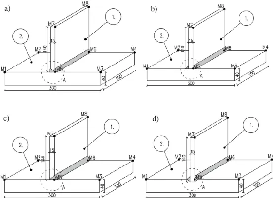
Small scale welded T-joints (Figure 1) of a stator segment of a wind turbine are investigated in the current study. The major aim of the experimental research program is to evaluate the effect of different filler metals, welding variables and types of welding joints on productivity and the structural behaviour. High-cycle fatigue is crucial in case of wind turbines, therefore, four types of joints are analysed (Figure 2) having considerably different resistance against cyclic loading: (i) double-beveled butt weld, (ii) double-sided fillet welds, (iii) single-beveled butt weld and (iv) a novel T-joint using a groove and double-sided fillet welds. Number of weld passes and heat input per unit length are the

investigated variables resulting in a database of input parameters including the cross sectional area of the fusion zones. It is the basis of the heat source model verification.

Thirty-six welded specimens are manufactured altogether. The following notations are used for the joints (e.g., JTX-Y-0Z): JT – T-joint; X – 1/2/3/4 – double-beveled butt weld/double-sided fillet welds/single-beveled butt weld/novel T-joint using a groove, with a groove angle of 90°, and double-sided fillet welds; Y – 1/2 – solid wire/flux cored electrode; Z – number of specimen. All the specimens are made from S355J2+N steel grade with a length of 100 mm. Base plates are manufactured from steel plates with dimensions of 300 × 100 × 40 mm, while stiffeners have dimensions of 140 × 100 × 15 mm. Plasma cutting is used for carving the plates. A Fronius TransPuls Synergic 5000 welding power source, M21 - ArC - 18 (Corgon 18) shielding gas and PA flat or PB horizontal-vertical welding positions are used for metal active gas (MAG) welding. Solid wire (Esab OK Aristorod 12.50) and flux cored (Böhler Ti52 T-FD) electrodes with diameters of 1.2 mm are used during manufacturing. Preheat and interpass temperatures are both 150 °C.

Ambient temperature is between 20-22 °C during the experiments. Heat input per unit length varies between 6.01 and 26.94 kJ/cm depending on filler metal, joint type and number of passes.

Fig. 1 Tack welded T-joints before welding.

Fig. 2 Types of investigated joints: (a) double-beveled butt weld, (b) double-sided fillet welds, (c) single-beveled butt weld and (d) a novel T-joint using a groove and double-sided fillet welds.

The initial and deformed configurations of the joints are measured with a coordinate- measuring machine in specific points, denoted with M1-M8 in Figure 2, thus, welding- induced deformations can be calculated after using common coordinate transformations.

Temperature is measured by a thermocouple and an infrared thermal camera during welding. The camera uses a fix value for emissivity, therefore, a code is developed to calibrate the measurements of the camera using data recorded by the thermocouple. The measurement range of Type K (Chromel/Alumel) thermocouples is -200 °C – 1200 °C, while the sensitivity is around 41 µV/°C. Thermoelectric voltages are converted to temperatures via a Thermo-MXBoard thermocouple adapter and a QuantumX MX840A data acquisition system, that operates as a universal amplifier. The temperature variation in time is plotted in, therefore, real-time monitoring of fixed points is possible during experiments. A ThermoPro^TM TP8S infrared thermal camera with high-temperature filter is part of the measurement system as well. It uses a focal plane array uncooled microbolometer with 384 × 288 pixels. Its spectral range is 8 – 14 μm, while its sensitivity is 0.08 °C at 30 °C. The measurement range is -200 °C – 2000 °C, whilst the operating temperature is between -20 °C and 60 °C. Basically, it is only capable of recording static thermal images that can be analysed in its program. It is not sufficient for time-dependent analysis, therefore, an approach is developed. A video capture card digitizes the composite video signal via Image Acquisition Toolbox in MATLAB R2016b [27]. A code is

a) b)

c) d)

developed to record videos, hereafter the .AVI videos are split into frames. Frames can be analysed regarding the red, green and blue (RGB) colour code, because the temperature palette unequivocally determines actual temperature values for each pixel. Spot and time- temperature curve analysis are implemented in the code for further data processing. The calculated virtual temperatures are calibrated according to thermocouple measurements, thus, a temperature scaling is necessary. The principle of scaling is having the same computed areas under each curve, thereunto trapezoidal rule integration is used. Surface and material properties can be handled easily, while the temperature-dependent emissivity is also taken into consideration. The cross sectional area of the fusion zone is measured after fabrication using macrographs. Vickers hardness tests and microstructural analyses are also carried out.

EXPERIMENTAL RESULTS

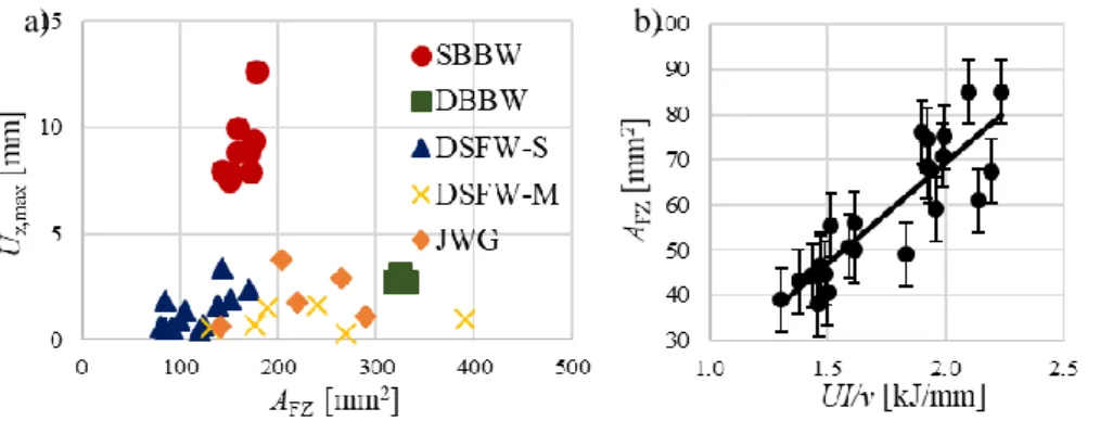
Welding variables, such as voltage, current, travel speed, are registered during welding, therefore, total heat input per unit length can be calculated. The deformations due to welding differ in a great extent in case of the presented types of joints, as the number of weld passes, total heat input and single/double sided welding have a large influence on residual strains. The most important component of deformations is the transverse deformation of the top due to angular distortion; the base plates are much stiffer, thus, vertical deformations are quasi-zero. Maximum Ux,max transverse deformations of the top and the AFZ cross sectional area of the fusion zone for every single case is shown in Figure 3; measurements are sorted in groups regarding the types of the joints. A linear regression analysis is carried out using the least squares method to determine the relationship between AFZ and the UI/v total heat input per unit length, marked with continuous solid line, for double-sided fillet welds with single weld passes. Measurements and derived heat input data are showed in Figure 3 as well. Error bars are denoting the s = 7.05 mm² standard deviation of discrepancies between measured data and corresponding values of the regression line due to uncertainties in welding variables as arc length and travel speed are not constant during welding.

Fig. 3 Fusion zone size vs. a) maximum transverse deformations of the top and b) net heat input.

a) b)

Maximum transverse deformations of the top are evaluated regarding the joint type and the cross sectional area of fusion zone. Specimen JT3-1-03 with single-beveled butt weld (SBBW) has not been taken into account in the assessment process as tack welds have fractured during transportation. The plates are repositioned and new tack welds are laid, therefore, the measurements of the deformed configuration cannot be used for deformation calculations, it would be erroneous. In addition, JT1-2-01, JT1-2-02 and JT1-2-03 T-joints are manufactured with single-bevel butt welds instead of double-beveled butt welds (DBBW), hence, they are treated as JT3 specimens. An obvious trend cannot be determined in case of multi-pass welding of double-sided fillet welds (DSFW-M) and double-beveled butt welds due to insufficient data. Larger transverse deformations and heat input are characteristic for larger fusion zones in case of joints with groove (JWG) and double-sided fillet welds with single weld passes (DSFW-S) regarding the whole joint.

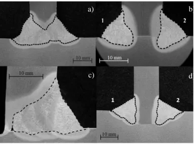
The cross sectional areas of fusion zones are measured after manufacturing using macrographs. Typical macrographs and fusion lines, denoted by dashed lines, are introduced in Figure 4 for a double-beveled butt weld, double-sided fillet welds, a single- beveled butt weld and a novel T-joint using a groove and double-sided fillet welds.

Fig. 4 Typical macrographs of joints: (a) double-beveled butt weld, (b) double-sided fillet welds, (c) single-beveled butt weld and (d) a novel T-joint using a groove and double-sided fillet welds.

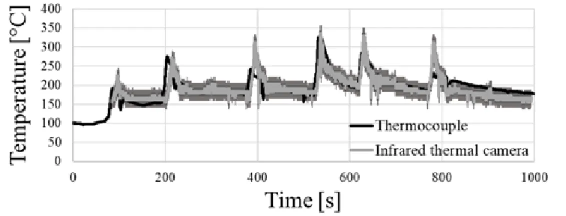
Thermal cycles are determined for six specimens using a thermocouple located 15 mm far from the stiffener in transverse direction and positioned in the centre longitudinally.

Virtual temperatures of the infrared camera are calibrated according to thermocouple measurements via temperature scaling for different temperature ranges. Figure 5 shows temperature measurements for JT4-2-02, while error bars are denoting the s = 20.6 °C standard deviation of temperature differences derived from the two approaches. Hereafter, temperature scaling factors can be used for other specimens, hence, solely infrared thermal camera is applied for further weldments.

a) b)

c) d)

Fig. 5 Temperature measurements of a thermocouple and the calibrated infrared thermal camera.

Vickers hardness tests and microstructural analyses are also carried out for eight specimens (two for each type of welding joint). A ferritic and pearlitic microstructure is specific for the base material; its hardness varies between 153 and 173 HV. The highest hardness values are measured at the boundary of the heat-affected zone and the fusion zone;

the maximum values are between 253 and 363 HV. A significant decrease of 30-110 HV can be observed in the fusion zone. The fusion zone contains ferrite, pearlite and bainite, while a ferritic and pearlitic microstructure is typical for the heat-affected zone with bainitic patterns in some cases. Cooling rate is lower in the weld pool and on its surface then in the heat-affected zone. The so-called Δt8/5 cooling time, that is necessary for cooling from 800

°C to 500 °C, has to be shorter for the base plate as higher hardness values are measured, in the corresponding heat-affected zone, then in the stiffener. There is no significant difference in hardness between face and root side, except in case of single-beveled butt welds naturally. The type of filler metal does not have any notable influence on hardness in these cases. Hardness profiles of double-sided fillet welds and joints with grooves do not differ in a great extent. Hardness profiles for face and root sides and the points used for measurements are presented in Figure 6.

Fig. 6 a) A typical hardness profile and b) points for measurements.

The weldments are manufactured by using a Fronius TransPuls Synergic 5000 welding power source for MAG welding using constant-voltage (slightly drooping) characteristics.

a) b)

Direct current and reverse polarity (DC+) are applied for the current applications. Welding current (I) and voltage (U) are registered during welding, thus, the operating points for each weld pass, assuming that arc length is constant, can be determined for configuration with solid wire and flux cored electrodes as arc characteristics for different filler metals, wire diameters and shielding gases are distinct. The solid wire electrode is an Esab OK Aristorod 12.50 (EN ISO 14341-A G 42 4 M G3Si1) and the flux cored electrode is a Böhler Ti52 T- FD (EN ISO 17632-A T 46 4 P M 1 H5). Diameter of electrodes is 1.2 mm, while shielding gas is EN ISO 14175 - M21 - ArC - 18. Eighty-two weld passes are laid using solid wire electrodes and eighty-one weld passes are carried out applying flux cored electrodes, hence, the number of data points is equal to the number of weld passes in Figure 7. A linear regression analysis is carried out using the least squares method to determine the welding current-voltage relationship for globular and spray arc metal transfer modes, marked with continuous solid lines, for both electrodes. Error bars are denoting the s = 0.81 V and s = 0.38 V standard deviations, for solid wire and flux cored electrodes, of discrepancies between measured data and corresponding values of the regression line representing the uncertainties in arc characteristic ranges, i.e., increase and decrease of contact tip-to- workpiece distance and arc length.

Fig. 7 Operating points and working conditions for solid wire and flux cored electrodes.

The current-voltage equations of the solid lines for the solid wire and flux cored electrodes are

𝑈_{𝑠𝑜𝑙𝑖𝑑}(𝐼) = 0.103𝐼 − 0.45 (1)

𝑈_{𝑓𝑙𝑢𝑥}(𝐼) = 0.02318𝐼 + 17 (2)

representing the operating points after the linear regression analysis. These equations can be applied in the preliminary design phase when calculating heat input. In addition, they are implemented in the numerical model developed for the welding simulation of T-joints.

NUMERICAL APPROACH

A complex finite element framework has been developed in ANSYS 17.2 [28] to simulate welding processes for civil engineering and mechanical engineering applications.

Uncoupled transient thermo-mechanical analysis is performed, which is a comprehensive technique for welding simulations that is used for determining and evaluating temperature fields, residual stresses and deformations. The most important features of the method implemented in the code are presented hereunder.

Uncoupled thermomechanical analysis means that calculated temperature fields are applied as nodal loads in the subsequent mechanical analysis. The typical couplings in a thermo-metallurgical-mechanical analysis (Figure 8) according to Refs. [1,3,29] are listed below; weak couplings and phase transformation-related phenomena are not taken into account in this paper:

1a Thermal expansion depends on microstructure of material.

1b Volume changes due to phase transformations.

1c Elastic and plastic material behaviour depend on microstructure.

1d Transformation-induced plasticity.

2a Microstructure evolution depends on deformation (weak coupling).

2b Phase transformations depend on stress state (weak coupling).

3a Thermal material properties depend on microstructure.

3b Latent heats due to phase transformations/solidification/melting.

4 Microstructure evolution depends on temperature.

5a Deformation evolution depends on temperature.

5b Mechanical material properties depend on temperature.

6a Deformation changes thermal boundary conditions (weak coupling).

6b Heat due to thermal, elastic and plastic strain rate (weak coupling).

Fig. 8 Couplings in a thermo-metallurgical-mechanical analysis.

In the current study, solid elements are used in the finite element model. SOLID70, a thermal solid element, has a three-dimensional thermal conduction capability. The element has eight nodes with a single thermal degree of freedom at each node. It allows for prism,

tetrahedral and pyramid degenerations when used in irregular regions. In the mechanical analysis SOLID185 is used as an equivalent structural solid element, which has eight nodes with three translational degrees of freedom (in nodal x, y, and z directions) at each node.

Thermal boundary conditions are defined for heat flow calculations. The initial temperature (room temperature or preheating temperature) of nodes is specified before the first load step of the thermo-metallurgical analysis. Nodal temperatures of not yet deposited weld passes are prescribed in the first step of the calculation to avoid ill-conditioned matrices. A combined temperature-dependent heat transfer coefficient of h_cr( )T is defined in the Function Editor of ANSYS to model the effect of convection and radiation to ambient in the developed code as described in Eqn. (3). In the equation below

2 2 2

( ) ( ) ( ) ( ) ( )

cr c amb amb

h T =h T +  T T+T T +T (3)

where h T_c( )is convective heat transfer coefficient or film coefficient,

T

is absolute surface temperature, T_amb is absolute ambient temperature,  is the Stefan-Boltzmann constant and ( ) T is emissivity. The film coefficient is assumed to be 25 W m^-2 K^-1, while emissivity is taken as a temperature-independent value with a magnitude of 0.8 in the current research. On the other hand, moving volumetric heat sources induce heat generation which is defined as element body force load during the transient thermo-metallurgical analysis. The double ellipsoidal heat source model is implemented in the current study.

Eqns. (4) and (5) determine the power density distribution in the front and rear quadrants, respectively

max

2 2 2

2 2 2

3 3 3

( , , )

f

x y z

cf a b

q x y z q e

− − −

=  (4)

max

2 2 2

2 2 2

3 3 3

( , , )

r

x y z

cr a b

q x y z q e

− − −

=  (5)

where characteristic parameters

c

_f , c_r ,

b

and a represent the physical dimensions of the heat source model in each direction shown in Figure 9, while q_max, maximum power density, is used for numerical scaling of power density, thus, the law of conservation of energy is fulfilled and heat generation error due to mesh formulation can be zeroed out in the transient analysis at every time step. The size of front and rear ellipsoids could be calibrated and fitted separately, while it could be applied even to simulate deep penetration welding. Several analogous functions exist to describe the power density distribution of a double ellipsoidal heat source, e.g., Bradac [30] used different constants in the exponent for each direction instead of a value of 3. Due to lack of sufficient data, Goldak, Chakravarti and Bibby [21] assumed that it is reasonable to take the distance in front of the source equal to one half of the weld width (

c

_f

= a

) and the distance behind the source equal to twice the weld width (c_r =4a) as a first approximation. The idea of using a double ellipsoidal heat source model instead of a single ellipsoidal one is explained by Goldak [31] as an attempt to generate typical weld pool shapes capturing the ‘digging action of the arc’ in front and

‘slower cooling of the weld by conduction of heat into the base metal’ at the rear. In general,

it is recommended by Goldak et al. [32] that the heat source may not move more than half of the weld pool length to function appropriately in three-dimensional welding simulations using the transient method.

Fig. 9 Notation and power density distribution of the double ellipsoidal heat source model.

In the mechanical analysis temperature fields are applied as nodal loads as explained before. Clamping conditions (i.e., rotational and translational degree of freedom constraints) have an important impact on the evolution of deformations and stresses. Even the release time of clamps has an appreciable influence on residual stresses and deformations. First of all, rigid body motion has to be avoided. Therefore, defining the minimum number of constraints is necessary to analyse a statically determinate structure.

In addition, clamps can fundamentally act like rigid (or elastic) supports. In case of statically indeterminate structures, the additional constraints have to be deleted in an intermediate (hot release) or in the last sub-step (cold release) of the simulation to assess residual stresses and deformations.

Depending on the welding process, welded joints can be created with or without filler material addition. Therefore, initial gaps and deposited material have to be modelled in the welding simulation. The ‘birth and death’ procedure [28] is added in the thermal analysis.

Element activation and deactivation can be executed using the EALIVE and EKILL commands, respectively. EKILL uses a stiffness matrix multiplier of 10-6 (it can be changed via ESTIF command) by default for deactivated elements. In the mechanical analysis the quiet element technique [33] is implemented instead of ‘birth and death’

procedure presented previously, since all elements are active from the beginning of the calculation. Regarding the works of Refs. [34-35], extremely reducing Young’s modulus can cause numerical problems, therefore, a reduction of two orders of magnitude is sufficient. Therefore, the Young’s modulus of 1000 MPa is used for un-deposited material, while linear thermal expansion coefficient is temperature-independent and taken as zero to ensure thermal strain free bead elements before welding. Material model changes for weld bead elements only above 1200 °C as it is considered to be the reference temperature.

In the current investigation, material properties are based on EN 1993-1-2:2005 [36].

The code is basically recommended for structural fire design, but there are several examples (e.g., Refs. [6-8]) demonstrating its applicability for welding simulation purposes as well.

The material properties are defined between 20 °C and 1200 °C in the standard.

Temperatures can be much higher during welding, therefore, material properties are set as

constant values above 1200°C. Eurocode uses reduction factors for considering temperature dependent Young’s modulus, yield strength and stress-strain curves. This material model has a notable advantage: only yield strength (355 MPa in the current paper) and Young’s modulus are needed to be known on room temperature to describe the mechanical behaviour of the material. The required parameters are given in the Annex A of EN 1993-1-2 to describe stress-strain curves. It also gives a recommendation for modelling hardening below 400 °C. A multilinear isotropic hardening model is used in the simulations assuming a von Mises yield criterion. Large deflection effects are taken into account in the mechanical analysis.

RESULTS

SENSITIVITY ANALYSIS

The sensitivity analysis focuses on the effect of thermal efficiency and characteristic parameters of the heat source model. The dimensions of T-joints with double-sided fillet weld are identical to the experimental ones, while throat thickness is 5 mm. A gap of 0.5 mm filled with ‘un-deposited material’ is modelled between the base plate and the stiffener.

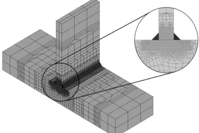
The model consists of 27010 finite elements (Figure 10). The minimum number of constraints are defined to analyse a statically determinate structure.

Fig. 10 Finite element model of a T-joint with double-sided fillet weld.

Interpass temperature is not controlled, the 2nd weld pass is laid right after the 1st weld pass with the same welding direction. Welding variables are I = 270 A, U is calculated using Eqn. (1) and v = 4 mm s-1. Ambient temperature is taken as 20 °C, while preheat temperature is 150 °C. The reference values for the characteristic parameters of Goldak’s double ellipsoidal heat source model are 𝑎 = 𝑏 = 𝑐_𝑓 = 2.5mm and 𝑐_𝑟= 4𝑐_𝑓. These parameters are scaled in the sensitivity analysis to investigate the effect of power density

distribution. Scaling factors of 1.00, 1.50, 2.00, 2.50 and 3.00 are applied; thermal efficiency is 1.00. Five additional analyses are performed in order to analyse the influence of thermal efficiency, which is increased in 0.10 steps from 0.60 to 1.00.

Figure 11 shows weld pool size and isothermal lines in the vicinity of the weld in the midsection during welding of the 1st weld bead. Arrows show increasing tendency of fusion zone size. Scaling the reference heat source parameters results in lower power density.

Thus, weld pool size decreases as scaling factor increases. Temperature does not even reach the liquidus temperature, assumed to be 1500 °C, in the weld bead elements when the scaling factor is equal to 3.00. The cross sectional area of the weld pool is 47.5 mm2, 45.5 mm2, 36 mm2, 12.5 mm2 and 0 mm2 for scaling factors of 1.00, 1.50, 2.00, 2.50 and 3.00, respectively. Variation of thermal efficiency has a similar effect as it has an influence on power density distribution; weld pool size increases as thermal efficiency increases. The cross sectional area of the weld pool is 25 mm2, 32 mm2, 37 mm2, 42.5 mm2 and 47.5 mm2 for thermal efficiency of 0.60, 0.70, 0.80, 0.90 and 1.00, respectively.

Fig. 11 Size of the fusion zone using heat source parameter scaling by a) 1.00, b) 1.50, c) 2.00, d) 2.50 and e) 3.00 and thermal efficiency of f) 0.60, g) 0.70, h) 0.80, i) 0.90 and j) 1.00.

Figure 12 sums up the transverse deformations of the joint after cooling. Configurations a)-e) have maximum transverse deformations of 1.56 mm, 1.46 mm, 1.26 mm, 0.93 mm and 0.45 mm, respectively. Transverse deformation of the stiffener decreases as scaling factor increases. Arrows show increasing tendency of deformations. For instance, scaling factor of 2.00 results in a 20% decrease in deformations in comparison to the reference configuration. Obviously, configurations d) and e) are erroneous as temperature just reaches the reference temperatures in the finite elements representing the weld bead (Figure 11), while the elevated temperature is lower than liquidus temperature in the corresponding finite elements. Configurations f)-i) have maximum transverse deformations of 1.41 mm, 1.46 mm, 1.54 mm, 1.58 mm and 1.56 mm, respectively. Transverse deformation of the stiffener slightly increases as thermal efficiency increases, however, the variation is within 10% due to 67% increase in thermal efficiency.

a) b) c) d) e)

f) g) h) i) j)

Fig. 12 Transverse deformations using heat source parameter scaling by a) 1.00, b) 1.50, c) 2.00, d) 2.50 and e) 3.00 and thermal efficiency of f) 0.60, g) 0.70, h) 0.80, i) 0.90 and j) 1.00.

Figure 13 shows the von Mises residual stresses in the vicinity of the weld beads in midsection after cooling. The plastic zones are shown in the figure, where the residual stress is higher than the yield strength, which is 355 MPa in this case. The same conclusions can be drawn as for Figure 11. Arrows show increasing tendency of plastic zone size. Plastic zone size decreases as the weld pool size decreases. The signs of lack of fusion is presented for configuration e) for instance, where several finite elements in the weld bead remains elastic, while the quasi-zero penetration is simulated in the joint. The gap, initially filled with un-deposited material, is the widest in this case as practically the material is not melted.

Results show that thermal efficiency and the scaling factor may have a similar effect on residual stresses and transverse deformations However, it is important to emphasize that sufficient power density is requisite to reach the reference temperature of un-deposited material, otherwise, the material model for weld bead elements remain elastic with a low Young’s modulus. It results in quasi-zero stresses in weld beads due to lack of fusion affecting overall residual stresses in conjunction with obtaining equilibrium of resultant internal forces and bending moments in any section of the specimen. On the other hand, 100% increase in scaling factor for the first three cases results in a variation of 32% in the weld pool size, while the variation is within 90% due to 67% increase in thermal efficiency.

Fig. 13 von Mises residual stresses using heat source parameter scaling by a) 1.00, b) 1.50, c) 2.00, d) 2.50 and e) 3.00 and thermal efficiency of f) 0.60, g) 0.70, h) 0.80, i) 0.90 and j) 1.00.

a) b) c) d) e)

f) g) h) i) j)

a) b) c) d) e)

f) g) h) i) j)

DETERMINATION OF THERMAL EFFICIENCY

Generally, thermal efficiency of a welding process can be evaluated using several approaches. In this study, the thermal efficiency is determined by the comparison of experimental and numerical data. Thermocouples and infrared thermal imaging are utilized to carry out temperature measurements during welding, as presented in section 3.2, thus, thermal cycles determined by finite element models can be compared with experimental data. In addition, macrographs are used to evaluate the thermal efficiency as well.

Nevertheless, the EN 1011-1:2009 standard [37] recommends to use 0.80 as thermal efficiency, while Radaj [29] introduced a range between 0.65-0.90 for metal active gas welding. The sensitivity analysis in the previous section shows that thermal efficiency has a larger effect on fusion zone size than scaling the characteristic parameters of the heat source, while the latter has a negligible effect on total (elastic and thermal) strains and temperatures further from the weld bead as presented by Kollár and Kövesdi [8].

T-joints with double-sided fillet weld (JT2-1-06 and JT2-2-02 welded with flux cored and solid wire electrodes, respectively) are chosen for the determination of thermal efficiency. The actual dimensions of the joints, which are measured, are modelled with the corresponding throat thicknesses. Throat thicknesses are measured on the macrographs for the weld beads which are single pass welded; models are built up with average throat thicknesses. The 2^nd weld pass is laid after the 1^st weld pass with opposite welding direction.

Welding variables are summed up in Table 1 in section 5.3. Ambient temperature is taken as 20 °C, while preheat and interpass temperatures are both 150 °C. The characteristic parameters of Goldak’s double ellipsoidal heat source model are 𝑎 = 𝑏 = 10mm and 𝑐𝑟 = 𝑐_𝑓= 2.5 mm for both specimens. Nodes in the stiffener in the midsection, 10 mm above the base plate, are chosen for the comparison of experimental and numerical data (Figure 14).

Fig. 14 Determination of thermal efficiency by a) temperature measurements for flux cored and solid wire electrodes and b) a macrograph of specimen JT2-1-06.

Figure 14 shows the time-temperature curves based on infrared thermal imaging (‘Measurement’) and the finite element analysis (FEA). The peak temperature is

a) b)

approximately 700-800 °C for both cases and the cooling phenomenon is also simulated successively. The temperature is about 200 °C at 200 s in case of the investigated configurations for both approaches. The figure sums up the macrograph of the JT2-1-06 specimen as well and a cross section of the finite element model showing the fusion zone (and the heat-affected zone in case of the macrograph). The basis of calibration is related to the fusion zone size. The aim is to approximate the measured fusion zone size within an arbitrary ±10% range specified for treating uncertainties in welding variables (the same way as it is treated in the relationship between welding current and voltage in section 3.2).

The cross sectional areas of the fusion zones for JT2-1-06, by measurements, are 76 mm2 and 75 mm2 for the 1st and 2nd weld beads, respectively. In addition, fusion sizes are 43 mm2 and 39 mm2 for JT2-2-02. The corresponding simulated weld pool sizes are 77 mm2, 72 mm2, 42 mm2 and 37 mm2, respectively, which are within the reasonable range.

According to the results of the sensitivity analysis the influence of thermal efficiency is already known in case of the actual T-joint, therefore, thermal efficiency was changed in 0.10 steps. Thermal efficiency of 0.90 is accepted related to the comparison of numerical and experimental data and it is applied in the simulations hereafter for both electrodes; in addition, it is in conjunction with the values published in Ref. [29] mentioned before.

CALIBRATION AND VERIFICATION OF THE DOUBLE ELLIPSOIDAL HEAT SOURCE MODEL

In this section, the characteristic parameters of the implemented double ellipsoidal heat source model are calibrated for a typical range of welding variables in case of double-sided fillet welds with single weld passes. The developed welding process model for welding simulation of double-sided fillet welds with single weld passes is verified. A total of twelve specimens are modelled.

Double-sided fillet welded T-joints with single pass welds are investigated. The actual dimensions of the joints, which are measured, are modelled with the corresponding throat thicknesses. The parametric model of section 5.2 is used in the simulations. The 2^nd weld pass is laid after the 1^st weld pass with opposite welding direction. Ambient temperature is taken as 20 °C, while preheat and interpass temperatures are 150 °C. Table 2 sums up specimen notations, # number of weld pass, type of filler metal, I welding current, U voltage, v travel speed, a characteristic parameter, q = ηUI/v net heat input per unit length, AFZ and AFZ,FEA fusion zone sizes based on measurements and numerical analyses and error in simulated fusion zone size, respectively. Voltage is calculated using Eqns. (1) and (2) depending on the type of filler metal. After performing dozens of iterations a function of heat input per unit length is developed to evaluate a and

b

characteristic parameters. The a

and

b

characteristic parameters for JT2-2-02 are outliers (bold letters) in data, therefore, the specimen is ignored when a(q) polynomial function is approximated. The AFZ,FEA fusion zone sizes in the table are determined by characteristic parameters using Eqn. (6),

11.094 3 62.383 2 117.52 60.8

) 1

( q q q 2

a q = − + − [mm];

c

_r

= = c

_f

2.5

mm (6)

for flux cored electrodes. The model for this configuration assumes that

a b =

and 𝑐_𝑟 = 𝑐_𝑓= 2.5 mm regarding previous simulations of the joints. The characteristic

parameters of Goldak’s double ellipsoidal heat source model are independent of the q net heat input per unit length for the configurations welded with solid wire electrode (𝑎 = 𝑏 = 10mm and 𝑐𝑟= 𝑐𝑓= 2.5mm). Obviously, the small c_rand 𝑐𝑓 parameters result in a requirement of dense mesh along welding trajectory.

Table 2 Input and output data for the calibrated cases.

Specimen # Filler metal

I [A]

U [V]

v [mm/s]

q [kJ/mm]

a [mm]

AFZ

[mm²] AFZ,FEA

[mm²]

Error [%]

JT2-1-01 1 solid wire 305 30.97 +4.77 1.78 10 76 77 1.3

2 solid wire 280 28.39 -4.17 1.72 10 75 72 -4.0

JT2-1-02 1 solid wire 280 28.39 +4.00 1.79 10 71 73 2.8

2 solid wire 261 26.43 -3.85 1.61 10 68 65 -4.4

JT2-1-03 1 solid wire 239 24.17 +3.70 1.40 10 55 51 -7.3

2 solid wire 229 23.14 -3.33 1.43 10 50 49 -2.0

JT2-1-04 1 solid wire 315 32.00 +4.17 2.18 10 85 87 2.4

2 solid wire 315 32.00 -4.55 1.99 10 85 83 -2.4

JT2-1-05 1 solid wire 221 22.31 +2.13 2.08 10 61 67 9.8

2 solid wire 221 22.31 -2.32 1.91 10 59 64 8.5

JT2-1-06 1 solid wire 270 27.36 +4.00 1.66 10 69 67 -2.9

2 solid wire 270 27.36 -4.00 1.66 10 74 68 -8.1

JT2-2-01

1 flux

cored 282 23.54 +2.92 2.05 13.5 67

68 1.5

2 flux

cored 282 23.54 -4.00 1.49 12.5 56

51 -8.9

JT2-2-02

1 flux

cored 210 21.87 +2.94 1.41 10.0 43

40 -7.0

2 flux

cored 210 21.87 -3.33 1.24 10.0 39

35 -10.3 JT2-2-03

1 flux

cored 311 24.21 +5.00 1.36 11.5 45

48 6.7

2 flux

cored 311 24.21 -5.00 1.36 11.5 47

49 4.3

JT2-2-04

1 flux

cored 265 23.14 +4.17 1.32 11.2 41

42 2.4

2 flux

cored 265 23.14 -4.35 1.27 10.5 44

43 -2.3

JT2-1-05

1 flux

cored 232 22.38 +3.57 1.31 11.0 38

39 2.6

2 flux

cored 232 22.38 -3.70 1.26 10.5 43

41 -4.7

JT2-1-06

1 flux

cored 311 24.21 +4.55 1.49 12.5 51

51 0.0

2 flux

cored 270 23.26 -4.17 1.36 11.5 49

46 -6.1

Figure 15 shows a nomogram for the developed approach. Selecting welding current, this may be wire feed rate for MIG/MAG welding power sources, determines voltage for solid wire or flux cored electrodes. Typical travel speeds and corresponding net heat inputs per unit length are shown as well for the two types of filler metals. Finally, characteristic parameters are evaluated using the curves of the figure or Eqn. (6). The U(I), a(q) and b(q) equations are implemented in the finite element code for further parametric studies and the sustainable virtual manufacturing of stator segments of a wind turbine as a final application in the future.

Fig. 15 Workflow of determining characteristic parameters for virtual manufacturing.

VALIDATION OF THE WELDING PROCESS MODEL

Calibration and verification of the heat source model makes it possible to investigate the effect of additional parameters and variants in qualitative and quantitative parametric studies and virtual prototyping. It is a time-consuming method, while there is a large amount of waste during the ’trial and error’ approach in the product development phase. Developing a sustainable virtual manufacturing process is an innovative way to reduce waste in workshops and specify optimal conditions depending on the requirements for advanced applications.

The verified parameters for double-sided fillet welds with single weld passes are validated using an extended set of parameters in case of the four types of T-joint; one from each configuration is presented in this paper. Figure 16 shows the finite element models of the weldments contributing in the validation process, while welding sequence is also denoted. T-joints with double-beveled butt weld (JT1-1-03), with double-sided fillet welds using multiple passes (JT2-1-07), with single-beveled butt weld (JT3-2-01) and a novel configuration with groove (JT4-2-01) are studied. Models consist of 26052, 23112, 18632 and 23640 finite elements, respectively.

Table 3 sums up specimen notations, # number of weld pass, type of filler metal, I welding current, U voltage, v travel speed, denoting (+) positive and (-) negative welding directions, a characteristic parameter, q = ηUI/v net heat input per unit length, AFZ and AFZ,FEA fusion zone sizes based on measurements and numerical analyses and error in simulated fusion zone size, respectively. Voltage is calculated using Eqns. (1) and (2) depending on the type of filler metal. Fusion zone sizes in the table are related to the whole joints as multi-pass welding is used for the weldments. Welding sequence is summed up in Figure 17 for the investigated cases.

Table 3 Input and output data for the validated cases.

Specimen # Filler metal I

[A]

U [V]

v [mm/s]

q [kJ/mm]

a [mm]

AFZ

[mm²] AFZ,FEA

[mm²]

Error [%]

JT1-1-03

1 solid wire

190 19.12 +3.57 0.92 10

331

(298) 302 -8.8 (1.3) 2 solid

wire

280 28.39 +4.55 1.57 10 3 solid

wire

280 28.39 +5.26 1.36 10 4 solid

wire

270 27.36 +5.26 1.26 10 5 solid

wire

280 28.39 -3.33 2.15 10 6 solid

wire

280 28.39 -4.17 1.72 10 7 solid

wire

270 27.36 -5.56 1.20 10

JT2-1-07

1 solid wire

278 28.18 +8.33 0.85 10 95 + 94

86 + 100

-1.3 2 solid

wire

262 26.54 +7.69 0.81 10 3 solid

wire

276 27.98 -3.85 1.81 10 4 solid

wire

278 28.18 -3.45 2.04 10

JT3-2-01

1 flux

cored 260 23.03 +3.85 1.40 11.9

158 163 3.2

2 flux

cored 238 22.52 +3.13 1.54 12.7 3 flux

cored 245 22.68 +5.00 1.00 5.4 4 flux

cored 242 22.61 +4.17 1.18 9.2 5 flux

cored 242 22.61 +4.17 1.18 9.2

JT4-2-01

1 flux cored

270 23.26 +5.88 0.96

4.4 69 + 72

67

+73 -0.7 2 flux

cored

270 23.26 +4.17 1.36

11.5 3 flux

cored

270 23.26 +4.35 1.30

10.9 4 flux

cored

270 23.26 +5.00 1.13

8.3

Fig. 16 Finite element models of a) JT1-1-03, b) JT2-1-07, c) JT3-2-01 and d) JT4-2-01.

Figure 17 shows the simulated fusion zones and the macrographs highlighting fusion lines with dashed lines; liquidus temperature is assumed to be 1500 °C. Measurements and numerical results are in a good agreement for the specimens, the absolute maximum error in the cross sectional area of the fusion zone is 8.8%, which is a quite convincing result.

Namely, the calibrated and verified double ellipsoidal heat source model is validated for multi-pass welding using an extended set of parameters. The largest discrepancy comes forward in case of JT1-1-01, which is T-joint with a double-beveled butt weld. However, the complex geometry of weld face is not taken into account in the simulations. Neglecting the difference between the perfect and imperfect weld geometry reduces the difference to 1.3% as the measured fusion zone size becomes 298 mm². On the other hand, geometry of weld face does not have a large influence on results for the other T-joints.

Fig. 17 Simulated and measured fusion zones for a) JT1-1-03, b) JT2-1-07, c) JT3-2-01 and d) JT4-2-01.

a) b)

c) d)

a) b) c) d)

Figure 18 sums up the total deformations of the joints after cooling. Specimens a)-d) have maximum transverse deformations of 2.82 mm, 1.26 mm, 8.61 mm and 1.07 mm, respectively. Results show that the novel T-joint, using a groove and double-sided fillet weld, has performed well in a distortion controlled design. Obviously, the T-joint with single-beveled butt weld is the worst configuration in this sense. On the other hand, it is important to highlight that throat thickness varies for the four specimens.

Fig. 18 Simulated and measured fusion zones for a) JT1-1-03, b) JT2-1-07, c) JT3-2-01 and d) JT4-2-01.

The top nodes, representing the maximum transverse deformations and denoted with an

‘x’ mark in Figure 18, are selected and typical thermal and displacement data as a function of time are also given in Figure 19 to show the importance of different joint configurations.

The time limit in the figure is maximized in 1500 s for clarity, however, cooling to room temperature is modelled. Temperature is 150 °C in the first load step due to the preheat temperature. Welding time varies in a function of travel speed and number of weld passes for the validated cases. Transverse nodal displacement decreases after the 4^th weld pass for JT1-1-03 and it is alternating for JT2-1-07 and JT4-2-01 because of the welding sequence shown in Figure 16. Obviously, transverse nodal displacement increases permanently during welding for the JT3-2-01 specimen which is a T-joint with a single-beveled butt weld. Eventually, phenomena shown in the figure is an unambiguous explanation for the beneficial effect of alternating welding sequence in a distortion controlled design.

a) b) c) d)

2.82 1.26 8.61 1.07

  

