Weld process model for simulating metal active gas welding Dénes Kollár

(1)

ORIGINAL ARTICLE

Weld process model for simulating metal active gas welding

Dénes Kollár¹&Balázs Kövesdi¹&László Gergely Vigh¹&Sándor Horváth²

Received: 30 September 2018 / Accepted: 4 January 2019

#The Author(s) 2019

Abstract

Generally, optimum welding variables and conditions of manufacturing are currently mainly determined by experiments for standardized production. Virtual manufacturing and virtual testing of weldments using finite element method provide a sustainable solution for advanced applications. The aim of the current research work is to develop a weld process model, using a three- dimensional heat transfer model, to ensure general applicability for typical joints of stator segments of wind turbines as a final application. A systematic experimental research program, containing temperature measurements during welding, macrographs, and deformation measurements, is carried out on small-scale test specimens using different welding variables. In addition, a numerical study using uncoupled transient thermomechanical analysis is performed. The weld process model uses Goldak’s double ellipsoidal heat source model for a metal active gas welding power source. It describes the correspondence between heat source parameters and net heat input for two types of electrodes. The model is validated via cross-sectional areas of fusion zones and deformations based on experiments. The relationship between current and voltage is determined based on large number of experimental data; thus, selecting a wire type, travel speed, and voltage directly defines the heat source parameters of the weld process model.

Keywords Welding simulation . Heat source model . Validation . Metal active gas welding . Numerical simulation . Weld process model

1 Introduction

There is a remarkable industrial demand on speeding up and improving manufacturing processes. Lindgren [1] revealed that welding technologies are generally developed by performing experiments and tests on prototypes, while computational methods are still rarely used in the development process. It is a substantial expectation that simulations will complement experiments using the“trial and error”process for obtaining Welding Procedure Specifications as a final result. Namely, both residual stresses and deformations are evaluated in the design phase to optimize welded structures.

However, nowadays, deformations are usually in focus where- as residual stresses are of interest in subsequent phases.

In most of the cases, it is time efficient and economical to use computer-aided engineering opportunities rather than determining optimal parameters experimentally. Developing a sustainable virtual manufacturing process is an innovative way to reduce waste in workshops and specify optimal conditions depending on the requirements. Goldak and Akhlaghi [2] denoted that in the automotive industry the number of prototypes has been reduced from a dozen to one or two applying computer-aided engineering sources as powerful, ro- bust, and efficient tools. The general aim of computational welding mechanics is to set up reasonably precise methods and models that are capable of controlling and designing welding technologies whilst ensuring suitable performance [3]. Obviously, it is an overall aim to perform numerical simulations faster and easier than to carry out welding experiments, especially when dealing with large welded structures [4]. The welding simulation procedure can be implemented in full-scale modeling frameworks describing the entire manufacturing process including steel rolling, cold forming, thermal cutting, and machining [5]. An additional tremendous

* Dénes Kollár

kollar.denes@epito.bme.hu

1 Department of Structural Engineering, Budapest University of Technology and Economics, 3 Műegyetem rakpart,

Budapest H-1111, Hungary

2 Lakics Machine Manufacturing Ltd., 1 Izzó utca, Kaposvár H-7400, Hungary

https://doi.org/10.1007/s00170-019-03302-3

(2)

advantage of computational welding mechanics is comparing different variants in the design phase, while performing subsequent analyses on virtual specimens, such as buckling [6–8]

or fatigue analysis, is also a potential.

The determination of residual stresses and deformations is highly recommended for manufacturers as well as for de- signers. In the case of steel structures, there are often assembly difficulties and resistance problems due to large weld sizes, high heat inputs, or poor clamping conditions during manufacturing. These effects can result in large deformations and residual stresses, which can reduce the resistance of steel structural elements. Most of the standards, such as EN 1993-1- 5:2005 [9], give only approximations for the equivalent (or initial) geometrical imperfections. Nowadays, due to the im- provement of hardware and computational approaches, it is feasible to examine large-scale welded joints and structures in an adequately accurate way, but it has to be declared that com- putations still have boundaries.

The aim of the current research is to develop a weld process model based on Goldak’s double ellipsoidal heat source model. A systematic research program is carried out on small-scale specimens using different welding variables. The experimental research program contains temperature measurements during welding, macrographs, and deformation measurements after welding. In addition, a numerical study using transient thermomechanical analysis is performed. The research program focuses on the relationship of welding variables and heat source model parameters. Based on the large number of experimental data, e.g., fusion zone size and deformations, thermal efficiency and heat source model parameters are calibrated and verified. The weld process model provides the heat source parameters as a function of net heat input. The validated model is able to increase structural performance of welded joints, while reducing the need of further experiments in the workshop of steel manufacturer companies, such as in the case of the project partner, Lakics Machine Manufacturing Ltd.

The validation procedure can be used by other researchers as well, while the validated heat source parameters are applicable for a metal active gas welding power source and two electrode types. The developed validation process can have significant role in the case of robotic welding, where welding trajectory, heat input, travel speed, and quality can be controlled precisely.

2 Literature review

Experiments and measurements are intended to assist in get- ting acquainted with heat sources. There is a fundamental need for better understanding the influence of certain parameters and more precise approaches to predict the realistic behavior during welding. Mathematical models are used to en- hance the knowledge of heat sources taking distinct effects

into account. Generally, the aim is to model the heat source as accurate as it is necessary depending on one’s purpose.

Therefore, Goldak and Akhlaghi [2] classified five generations of weld heat source models. The fifth class is the newest and most complex. The older ones are considered as sub- classes of each newer generation as latter generations include the attributes of former models. Table 1 sums up the pros, cons, applicability, and the need for calibration of each weld heat source model generation. The literature review focuses on the second-generation weld heat source models as these are relevant for the presented finite element calculations. Heat source models can be generalized for welding processes in a parameter range. According to Lindgren [3], weld process models are coupling the physics of the problem, the power density distribution in the weld pool and welding process parameters. Sudnik et al. [10,11] set up such a model earlier for laser beam welding taking energy transport, vapor pressure, and capillary pressure as well into account. Weld process models have much importance as experiments can be combined or fully replaced by calibrated heat source models in the region of interest [12].

First-generation heat sources comprehend point, line, and plane heat source models. The development of instantaneous point heat source models for two- and three-dimensional heat flow, solving the heat flow differential equation for quasi- stationary state, is credited to Rosenthal [13] and Rykalin [14]. Rosenthal made a few assumptions such as (i) the energy input from the heat source is uniform and moves with a constant velocity along a trajectory; (ii) all the energy is deposited into the weld at a single point; (iii) thermal properties are temperature-independent; (iv) heat flow is governed by conduction, meanwhile radiation and convection are ignored; and (v) in addition, latent heats due to phase transformations and fusion/solidification are neglected. The temperature field far from the weld bead could be determined with acceptable ac- curacy, but the precision of these analytical approaches may decrease severely in the fusion zone and the heat-affected zone. On the other hand, quasi-stationary state may not even exist for welded structures with complex welding trajectories according to Goldak et al. [15]; thus, the utilization of first- generation weld heat source models is restricted.

Second-generation weld heat source models define distribution functions instead of solving Dirichlet problems of first- generation models. It is mainly applied in finite element analysis and is suitable to handle complex geometries, weld pool shapes, and welding trajectories, while temperature- dependent material properties, radiation and convection, phase transformations, and latent heats due to phase transformations, fusion, and evaporation can be taken into account.

These models have to fulfill solely the heat equation; thus, power density, prescribed flux, and prescribed temperature functions are in this class according to [2,16]. The first innovative conception was a distributed flux model developed by

(3)

Pavelic et al. [17] and Rykalin [18] to model weld pools without nail-head shape or deep penetration. The description of distributed flux models, e.g., normal Gaussian distributed surface heat source and bivariate Gaussian distributed surface heat source, is given in [2] in a detailed manner. Prescribed temperature model was used by, e.g., [19, 20]. Goldak, Chakravarti, and Bibby [21] presented power density functions to model even complex weld pool shapes for arc welding or laser beam welding. General power density functions of spherical, hemispherical, single ellipsoidal, and double ellipsoidal heat sources are gathered in [2,16] as well. Recently, hybrid heat source models [22–25] are also published, as combination of heat source models is feasible for non-conform cases.

The current paper uses Goldak’s double ellipsoidal heat source model, a second-generation weld heat source model, as a basis of weld process model development. The weld process model provides the parameters of the double ellipsoidal heat source as a function of net heat input. According to the authors’knowledge, such a weld process model has not been published yet. The validated model is applicable to a metal active gas welding power source and two electrode types. The aim is to increase structural performance of welded

joints, while reducing the need for further experiments in the workshop of steel manufacturer companies. A three- dimensional heat transfer model is used to ensure general applicability for typical joints of stator segments of wind turbines as a final application.

3 Experimental research program

Small-scale welded T-joints (Fig.1) of a stator segment of a wind turbine are investigated in the current study. The major aim of the experimental research program is to evaluate the effects of different filler metals, welding variables, and types of welding joints on productivity and structural behavior.

High-cycle fatigue is crucial in the case of wind turbines;

therefore, three types of joints are analyzed (Fig. 2) having considerably different resistance against cyclic loading: (a) double-bevel butt weld, (b) double-sided fillet welds, and (c) single-bevel butt weld.

A number of weld passes and heat input per unit length are the investigated variables resulting in a database of input parameters including the cross-sectional area of the fusion zones.

Fusion zone size is measured after fabrication using Table 1 Pros, cons, applicability, and the need for calibration of weld heat source model generations (WHSMG)

WHSMG Pros Cons Applicability/calibration

First Analytical solution Low computational cost

Distribution of energy☒ Constant material properties Phase transformations☒ Radiation and convection☒ Simple weldment geometry Straight weld path

Discontinuities in geometry☒ Constant travel speed Quasi-steady state heat transfer

Approximates temperature for finite, infinite, or semi-infinite bodies without discontinuities and nonlinearities

Supports optimizing welding variables Makes approximations on phase proportions and

hardness possible

Calibration is not really possible

Second Distribution of energy Nonlinear material properties Phase transformations Radiation and convection Complex weld path Complex weldment geometry Discontinuities in geometry Varying travel speed Unsteady state heat transfer Moderate computational cost

Fluid flow☒

Complex weld pool shapes☒/☑ FDM or FEM: handles nonlinearities

Realistic temperature fields outside of the weld pool Complex weld pool shapes using prescribed

temperature model or combination of surface and/or volumetric heat source models Calibration is needed

Third Stefan problem

Cauchy momentum equation Complex weld pool shapes Higher computational cost

Additional input data may be needed for pressure distribution of the arc, mass flow rate into the weld pool, and surface tension on the liquid surface

Can take welding positions into account Weld pool shape becomes output data Calibration is not needed

Fourth Fluid dynamics

Complex weld pool shapes

Mathematical difficulties High computational cost

FVM: droplet flow can be included;

Calibration is not needed Fifth Model of the arc is included

Magneto-hydrodynamics Complex weld pool shapes

Mathematical difficulties High computational cost

Most general heat source model generation Application is actually limited to researches Calibration is not needed

FDM, finite difference method;FEM, finite element method;FVM, finite volume method

(4)

macrographs and it is considered to be the basis of the heat source model validation process. The initial and deformed configurations of the joints are measured with a coordinate- measuring machine at specific points, denoted by M1–M8 in Fig.2; thus, welding-induced deformations can be calculated after using common coordinate transformations. Vickers hardness tests, microstructural analyses, and temperature measurements during welding are also carried out. Thirty welded specimens are manufactured altogether. The following notations are used for the joints (e.g., JTX-Y-0Z): JT—T-joint;X—1/2/

3—double-bevel butt weld with bevel angles of 45° and a root gap of 3 mm/double-sided fillet welds/single-bevel butt weld with a bevel angle of 45°;Y—1/2—solid wire/flux cored electrode;Z—number of specimen. All the specimens have a length of 100 mm. Base plates are manufactured from steel plates with dimensions of 300 × 100 × 40 mm³, while stiffeners have dimensions of 140 × 100 × 15 mm³. Plasma cutting is used for carving the plates. Steel grade is S355J2+N for base plates and stiffeners as well; the chemical composition is summed up in Table2according to the inspection certificate.

A Fronius TransPuls Synergic 5000 welding power source, M21 - ArC - 18 (Corgon 18) shielding gas, and PA flat or PB horizontal-vertical welding positions are used for metal active gas (MAG) welding. Solid wire (Esab OK Aristorod 12.50) and flux cored (Böhler Ti52 T-FD) electrodes with diameters of 1.2 mm are used during manufacturing. Preheat and

interpass temperatures are both 150 °C. Ambient temperature is between 20 and 22 °C during the experiments. The total heat input per unit length varies between 0.60 and 2.71 kJ/mm depending on filler metal, joint type, and number of passes.

Welding sequences are shown in Figs. 3 and 4 for all the specimens, while Tables3,4,5, and6sum up specimen notations; number of weld pass #; type of filler metal; welding currentI; voltageU; travel speedv, denoting (+) positive and (−) negative welding directions; total heat input per unit length q=UI/v, fusion zone sizeAFZbased on measurements using macrographs (Figs.5,6,7, and8); and maximum measured transverse deformationUx,max, respectively. Fusion zone sizes in the tables are related to the whole joint in several cases as multi-pass welding is used for multiple weldments. Welding variables, such as voltage, current, and travel speed, are registered during welding; therefore, total heat input per unit length can be calculated. Three of the double-bevel butt weld configurations are welded only on single side; however, these joints are also listed under the corresponding tables and the macrographs are shown in the corresponding figures.

The deformations due to welding differ in a great extent in the case of the presented types of joints, as the number of weld passes, total heat input, and single/double-sided welding have a large influence on residual strains. The most important com- ponent of deformations is the transverse deformation of the top due to angular distortion; the base plates are much stiffer;

thus, vertical deformations are quasi-zero. Maximum transverse deformationsUx,maxand the cross-sectional area of the fusion zoneAFZ for every single case are shown in Fig.9;

measurements are sorted in groups regarding the types of the joints. A linear regression analysis is carried out using the least squares method to determine the relationship betweenAFZand the total heat input per unit lengthq=UI/v, marked by continuous solid lines, for double-sided fillet welds with single weld passes. Measurements and derived heat input data are showed in Fig.9as well. Error bars are denoting the standard deviation of discrepancies (s= 7.58 mm²and 3.95 mm²for solid wire and flux cored electrodes, respectively) between measured data and corresponding values of the regression line due to uncertainties in welding variables as arc length and travel speed are not constant during welding. Nevertheless, the slopes of continuous lines are different, which means that the size of fusion zone is smaller in the case of flux cored Fig. 1 Tack welded T-joints before welding

Fig. 2 Types of investigated joints:a) double-bevel butt weld,b) double-sided fillet welds, andc) single-bevel butt weld

(5)

electrodes by using the same total heat input per unit length.

Different thermal efficiencies and the protective slag formed over the weld, which is removed when using flux cored electrodes, may be an explanation of the discrepancies.

Maximum transverse deformations at the top of the specimens are evaluated regarding the joint type and the cross- sectional area of the fusion zone. Specimen JT3-1-03 with single-bevel butt weld (SBBW) has not been taken into account in the assessment process as tack welds have fractured during transportation. The plates are repositioned and new tack welds are laid; therefore, the measurements of the deformed configuration cannot be used for deformation calculations. In addition, JT1-2-01, JT1-2-02, and JT1-2-03 T-joints are manufactured with single-bevel butt welds instead of double-bevel butt welds (DBBW); hence, they are treated as JT3 specimens. An obvious trend cannot be determined in the case of multi-pass welding of double-sided fillet welds (DSFW-M) and double-bevel butt welds due to insufficient data. Larger transverse deformations and heat inputs are characteristic for larger fusion zones in the case of joints with double-sided fillet welds with single weld passes (DSFW-S) regarding the whole joint.

Temperature is measured by a thermocouple and an infrared thermal camera during welding. The camera uses a fixed value for emissivity; therefore, a code is developed to calibrate the measurements of the camera using data recorded by the thermocouple. The measurement range of Type K (Chromel/

Alumel) thermocouples is−200–1200 °C, while the sensitivity is around 41μV/°C. Thermoelectric voltages are converted to temperatures via a Thermo-MXBoard thermocouple adapter and a QuantumX MX840A data acquisition system, which operates as a universal amplifier. The temperature variation in time is plotted; therefore, real-time monitoring of fixed points is possible during experiments. A ThermoPro™TP8S infrared thermal camera with high-temperature filter is part of the

measurement system as well. It uses a focal plane array un- cooled microbolometer with 384 × 288 pixels. Its spectral range is 8–14 μm, while its sensitivity is 0.08 °C at 30 °C. The measurement range is−200–2000 °C, while the operating temperature is between−20 and 60 °C. The measured virtual temperatures (by the infrared thermal camera) are calibrated according to thermocouple measurements; thus, a temperature scaling is necessary. The principle of scaling is having the same computed areas under the curves, provided by the infrared camera at the same location as the thermocouple; thereunto, trape- zoidal rule integration is used. Surface and material properties could be handled easily, while the temperature-dependent emissivity is also taken into consideration.

Thermal cycles are determined for three specimens (JT1-2- 01, JT1-2-02, and JT1-2-03) using a thermocouple located 15 mm far from the stiffener in transverse direction and posi- tioned in the midsection longitudinally. Virtual temperatures of the infrared camera are calibrated according to thermocouple measurements via temperature scaling for different temperature ranges. Figure10shows temperature measurements for a specimen, while error bars are denoting thes= 20.6 °C standard deviation of temperature differences derived from the two approaches. Hereafter, temperature scaling factors can be applied at arbitrary points for further weldments when the infrared thermal camera is used.

Vickers hardness tests and microstructural analyses are also carried out for six specimens (two for each type of welding joint). A ferritic and pearlitic microstructure is specific for the base material; its hardness varies between 153 and 173 HV.

The highest hardness values are measured at the boundary of the heat-affected zone and the fusion zone; the maximum values are between 253 and 363 HV. A significant decrease of 30–110 HV can be observed in the fusion zone. The fusion zone contains ferrite, pearlite, and bainite, while a ferritic and pearlitic microstructure is typical for the heat-affected zone Table 2 Chemical composition of S355J2+N according to inspection certificate

C% Mn% Si% S% P% Cr% Ni% Al% Cu% Mo% Nb% V% Ti% N%

0.164 1.295 0.188 0.003 0.010 0.017 0.012 0.039 0.018 0.001 0.020 0.002 0.001 0.0038

a) b) c) d)

Fig. 3 Welding sequences fora)– b) double-bevel andc)–d) single- bevel butt welds

(6)

a) b) c) d)

Fig. 4 Welding sequences fora) single-pass andb)–d) multi-pass welding of double-sided fillet welds

Table 3 Welding variables, size of fusion zone, and maximum transverse deformation for double-bevel butt welds

Specimen # Filler metal I(A) U(V) v(mm/s) q(kJ/mm) AFZ(mm²) Ux,max(mm)

JT1-1-01 1 Solid wire 190 17.6 + 5.56 0.60 313 2.80

2 Solid wire 281 28.5 + 5.00 1.60

3 Solid wire 294 28.5 + 5.26 1.59

4 Solid wire 269 27.7 + 5.26 1.42

5 Solid wire 280 28.8 −3.33 2.42

6 Solid wire 280 28.8 −4.35 1.85

7 Solid wire 270 27.8 −5.56 1.35

JT1-1-02 1 Solid wire 190 18.6 + 4.35 0.81 323 3.09

2 Solid wire 187 18.5 + 4.76 0.73

3 Solid wire 246 25.1 + 5.56 1.11

4 Solid wire 270 27.8 + 5.00 1.50

5 Solid wire 280 28.8 −3.70 2.18

6 Solid wire 280 28.8 −5.00 1.61

7 Solid wire 270 27.8 −5.26 1.43

JT1-1-03 1 Solid wire 190 18.6 + 3.57 0.99 331 2.80

2 Solid wire 281 28.8 + 4.55 1.78

3 Solid wire 280 29.1 + 5.26 1.55

4 Solid wire 270 27.8 + 5.26 1.43

5 Solid wire 280 28.8 −3.33 2.42

6 Solid wire 280 28.8 −4.17 1.93

7 Solid wire 270 27.8 −5.56 1.35

JT1-2-01 1 Flux cored 240 22.8 + 4.17 1.31 150 7.50

2 Flux cored 260 23.5 + 4.35 1.40

3 Flux cored 250 23.3 −4.76 1.22

4 Flux cored 240 23.1 + 5.00 1.11

5 Flux cored 240 23 −5.26 1.05

JT1-2-02 1 Flux cored 260 23.5 + 3.85 1.59 171 7.89

2 Flux cored 240 22.7 + 4.00 1.36

3 Flux cored 240 22.7 −3.85 1.42

4 Flux cored 240 22.7 −4.55 1.20

5 Flux cored 240 22.7 −4.00 1.36

JT1-2-03 1 Flux cored 250 23 + 4.55 1.26 152 7.83

2 Flux cored 260 23.2 + 4.55 1.33

3 Flux cored 260 23.2 + 5.00 1.21

4 Flux cored 260 23.2 + 5.88 1.03

5 Flux cored 260 23.2 + 5.56 1.08

(7)

with bainitic patterns in some cases. Cooling rate is lower in the weld pool and on its surface than in the heat-affected zone.

The so-called Δt8/5 cooling time, which is necessary for cooling from 800 to 500 °C, has to be shorter for the base plate as higher hardness values are measured, in the corresponding heat-affected zone, than in the stiffener. There is no significant difference in hardness between face and root side, except in the case of single-bevel butt welds naturally.

The type of filler metal does not have any notable influence on hardness in these cases. Hardness profiles of double-sided fillet welds do not differ in a great extent. Hardness profiles of JT2-1-01 for face and root sides and the points used for measurements are presented in Fig.11.

The weldments are manufactured by using a Fronius TransPuls Synergic 5000 welding power source for MAG welding using constant voltage (slightly drooping) characteristics. Direct current and reverse polarity (DC+) are applied for the current applications. Welding current (I) and voltage (U) are registered during welding; thus, the operating points for each weld pass, assuming that arc length is constant, can be determined for configurations with solid wire and flux cored electrodes as arc characteristics for different filler metals, wire diameters, and shielding gases are distinct. The solid wire electrode is an Esab OK Aristorod 12.50 (EN ISO 14341- A G 42 4 M G3Si1) and the flux cored electrode is a Böhler Ti52 T-FD (EN ISO 17632-A T 46 4 P M 1 H5). The diameter of electrodes is 1.2 mm, while shielding gas is

EN ISO 14175 - M21 - ArC – 18 and gas flow rate is 12–15 l/min. Eighty-two weld passes are laid using solid wire electrodes and 81 weld passes are carried out applying flux cored electrodes; hence, the number of data points is equal to the number of weld passes in Fig. 12. A linear regression analysis is carried out using the least squares method to determine the welding current-voltage relationship for globular and spray arc metal transfer modes, marked with continuous solid lines, for both electrodes.

Error bars are denoting standard deviations of discrepancies (s= 0.81 V and s= 0.38 V), for solid wire and flux cored electrodes, between measured data and corresponding values of the regression line representing the uncertainties in arc characteristic ranges, i.e., increase and decrease of contact tip-to-workpiece distance and arc length.

The current-voltage equations of the solid lines for the solid wire and flux cored electrodes are

Usolidð Þ ¼I 0:103I−0:45 ð1Þ

Ufluxð Þ ¼I 0:02318Iþ17 ð2Þ representing the operating points after the linear regression analysis. These equations can be applied in the preliminary design phase when calculating heat input. In addition, they are implemented in the numerical model developed for the welding simulation of T-joints.

Table 4 Welding variables, size of fusion zone, and maximum transverse deformation for double-sided fillet welds (single- pass welding)

JT2-1-01 1 Solid wire 270 28.5 + 4.00 1.92 69 3.35

2 Solid wire 270 28.5 −4.00 1.92 74

JT2-1-02 1 Solid wire 221 20.6 + 2.13 2.14 61 0.46

2 Solid wire 221 20.6 −2.32 1.96 59

JT2-1-03 1 Solid wire 315 29.6 + 4.17 2.24 85 2.35

2 Solid wire 315 30.3 −4.55 2.10 85

JT2-1-04 1 Solid wire 239 23.5 + 3.70 1.52 55 1.36

2 Solid wire 229 23.5 −3.33 1.62 50

JT2-1-05 1 Solid wire 280 28.4 + 4.00 1.99 71 1.60

2 Solid wire 261 28.5 −3.85 1.93 68

JT2-1-06 1 Solid wire 305 29.7 + 4.77 1.90 75 1.87

2 Solid wire 280 29.7 −4.17 1.99 74

JT2-2-01 1 Flux cored 282 22.9 + 2.92 2.21 67 0.72

2 Flux cored 282 22.9 −4.00 1.61 56

JT2-2-02 1 Flux cored 210 20.9 + 2.94 1.49 43 1.82

2 Flux cored 210 20.5 −3.33 1.29 39

JT2-2-03 1 Flux cored 311 23.7 + 5.00 1.47 45 0.60

2 Flux cored 311 24 −5.00 1.49 47

JT2-2-04 1 Flux cored 265 23.6 + 4.17 1.50 41 0.58

2 Flux cored 265 23.6 −4.35 1.44 44

JT2-2-05 1 Flux cored 232 22.5 + 3.57 1.46 38 0.66

2 Flux cored 232 22.5 −3.70 1.41 43

JT2-2-06 1 Flux cored 311 23.9 + 4.55 1.63 51 0.88

2 Flux cored 270 23.3 −4.17 1.51 49

(8)

4 Numerical research program

A complex finite element model has been developed in ANSYS 17.2 [26] to simulate welding processes for civil engineering applications. Uncoupled transient thermomechanical

analysis is performed, which is a comprehensive technique for welding simulations that is used for determining and evaluat- ing temperature fields and residual stresses and deformations.

The most important features of the method implemented in the code are presented hereunder.

Table 5 Welding variables, size of fusion zone, and maximum transverse deformation for double-sided fillet welds (multi- pass welding)

JT2-1-07 1 Solid wire 278 27.9 + 8.33 0.93 94 + 95 1.53

2 Solid wire 262 27.9 + 7.69 0.95

3 Solid wire 276 27.8 −3.85 1.99

4 Solid wire 278 27.8 −3.45 2.24

JT2-1-08 1 Solid wire 276 28.3 + 6.67 1.17 114 + 125 1.63

2 Solid wire 257 28.2 + 6.67 1.09

3 Solid wire 267 28.2 −5.88 1.28

4 Solid wire 277 27.4 −6.25 1.21

5 Solid wire 262 26.5 + 5.56 1.25

6 Solid wire 259 26.5 −5.56 1.23

JT2-1-09 1 Solid wire 274 28.1 + 6.67 1.15 193 + 197 0.99

2 Solid wire 269 28.5 + 7.14 1.07

3 Solid wire 265 26.9 −7.69 0.93

4 Solid wire 262 27 −7.14 0.99

5 Solid wire 260 26.2 + 6.67 1.02

6 Solid wire 264 26.9 + 7.14 0.99

7 Solid wire 260 26.6 + 7.14 0.97

8 Solid wire 260 26.6 −6.67 1.04

9 Solid wire 255 26.6 + 7.69 0.88

10 Solid wire 260 26.6 −3.45 2.00

11 Solid wire 267 26.6 + 5.88 1.21

12 Solid wire 263 26.7 −5.88 1.19

JT2-2-07 1 Flux cored 270 23.9 + 6.67 0.97 63 + 68 0.58

2 Flux cored 270 23.9 + 8.33 0.77

3 Flux cored 270 23.9 + 4.55 1.42

4 Flux cored 266 23.8 + 5.26 1.20

JT2-2-08 1 Flux cored 253 23.1 + 6.25 0.94 90 + 86 0.72

2 Flux cored 253 23.1 + 7.14 0.82

3 Flux cored 245 22.8 + 5.88 0.95

4 Flux cored 248 22.7 + 6.25 0.90

5 Flux cored 245 22.8 + 5.88 0.95

6 Flux cored 245 22.4 + 4.76 1.15

JT2-2-09 1 Flux cored 240 22.3 + 5.88 0.91 133 + 136 0.32

2 Flux cored 235 22.1 + 6.67 0.78

3 Flux cored 242 22.2 + 7.14 0.75

4 Flux cored 242 22.2 + 7.14 0.75

5 Flux cored 242 22 + 6.25 0.85

6 Flux cored 242 22 + 6.25 0.85

7 Flux cored 242 22 + 6.67 0.80

8 Flux cored 241 22.4 + 5.88 0.92

9 Flux cored 231 22.5 + 5.88 0.88

10 Flux cored 248 22.7 + 6.25 0.90

11 Flux cored 240 22.7 + 6.25 0.87

12 Flux cored 249 22.6 + 5.88 0.96

(9)

Uncoupled thermomechanical analysis means that calculated temperature fields are applied as nodal loads in the subsequent mechanical analysis. The typical couplings in a thermo-metallurgical-mechanical analysis (Fig. 13) according to [1,3,27] are listed below; weak couplings and phase transformation-related phenomena are not taken into account in this paper:

1a Thermal expansion depends on microstructure of material.

1b Volume changes due to phase transformations.

1c Elastic and plastic material behaviors depend on microstructure.

1d Transformation-induced plasticity.

2a Microstructure evolution depends on deformation (weak coupling).

2b Phase transformations depend on stress state (weak coupling).

3a Thermal material properties depend on microstructure.

3b Latent heats due to phase transformations/solidification/melting.

4 Microstructure evolution depends on temperature.

5a Deformation evolution depends on temperature.

5b Mechanical material properties depend on temperature.

6a Deformation changes thermal boundary conditions (weak coupling).

6b Heat due to thermal, elastic and plastic strain rate (weak coupling).

In the current study, solid elements are used in the finite element model. A thermal solid element, SOLID70, with three-dimensional thermal conduction capability is applied Table 6 Welding variables, size

of fusion zone, and maximum transverse deformation for single- bevel butt welds

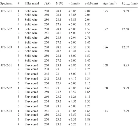
JT3-1-01 1 Solid wire 280 28.1 + 3.85 2.04 175 9.39

2 Solid wire 280 28.1 + 3.85 2.04

3 Solid wire 280 28.1 + 3.85 2.04

4 Solid wire 270 27.8 + 5.00 1.50

JT3-1-02 1 Solid wire 280 28.1 + 5.00 1.57 177 12.68

2 Solid wire 281 28.2 + 5.00 1.58

3 Solid wire 280 28.5 + 2.94 2.71

4 Solid wire 270 27.2 + 5.00 1.47

JT3-1-03 1 Solid wire 280 28.2 + 3.33 2.37 186 12.07

2 Solid wire 280 28.5 + 3.44 2.32

3 Solid wire 280 28.1 + 5.00 1.57

4 Solid wire 270 27.2 + 5.00 1.47

JT3-2-01 1 Flux cored 260 23.1 + 3.85 1.56 158 8.85

2 Flux cored 238 23 + 3.13 1.75

3 Flux cored 245 23 + 5.00 1.13

4 Flux cored 242 23.1 + 4.17 1.34

5 Flux cored 250 22.9 + 5.00 1.15

JT3-2-02 1 Flux cored 281 23 + 3.85 1.68 158 9.99

2 Flux cored 250 23.5 + 3.57 1.65

3 Flux cored 260 23.2 + 5.26 1.15

4 Flux cored 254 23.2 + 4.55 1.30

5 Flux cored 270 23.2 + 5.00 1.25

JT3-2-03 1 Flux cored 281 23 + 3.85 1.68 143 7.99

2 Flux cored 280 23.2 + 3.57 1.82

3 Flux cored 270 23.2 + 3.33 1.88

4 Flux cored 270 23.2 + 5.26 1.19

a) b) c) d) e) f)

Fig. 5 Macrographs of double-bevel butt welds:a)–c) JT1-1-01–JT1-1-03 andd)–f) JT1-2-01–JT1-2-03

(10)

for modeling the heat transfer problem. The element has eight nodes with a single thermal degree of freedom at each node. It allows for prism, tetrahedral, and pyramid degenerations when used in irregular regions. An equivalent structural solid element, SOLID185, is used in the mechanical analysis which has eight nodes with three translational degrees of freedom (in nodalx,y, andzdirections) at each node.

Thermal boundary conditions are defined for heat flow calculations. The initial temperature (room temperature or preheating temperature) of nodes is specified before the first load step of the thermo-metallurgical analysis. Nodal temperatures of not yet deposited weld passes are prescribed in the first step of the calculation to avoid ill-conditioned matrices. A combined temperature-dependent heat transfer coefficient hcr(T) is defined in the Function Editor of ANSYS [28] to model the effect of convection and radiation to ambient as described by Eq. (3). In the equation below

hcrð Þ ¼T hcð Þ þT σεð ÞT ðTþTambÞ² T²þTamb2 ð3Þ wherehc(T) is convective heat transfer coefficient or film coefficient,T is absolute surface temperature,Tamb is absolute ambient temperature, σ is the Stefan-Boltzmann constant, and ε(T) is emissivity. The film coefficient is assumed to be 25 W m⁻² K⁻¹, while emissivity is taken as a temperature-independent value with a magnitude of 0.8 in the current research. On the other hand, moving volumetric heat sources induce heat generation which is defined as element body force load during the transient thermo-metallurgical analysis. The double ellipsoidal heat source model is implemented in the current study.

Equations (4) and (5) determine the power density distribution in the front and rear quadrants, respectively

qfðx;y;zÞ ¼qmax⋅e⁻³^c^x^f²²⁻³^y

2

a2−3_b^z²2 ð4Þ

qrðx;y;zÞ ¼qmax⋅e⁻³^{cr 2}^x²⁻³^y^a²²⁻³^z^b²² ð5Þ where characteristic parameters cf, cr, b, and a represent the physical dimensions of the heat source model in each direction as shown in Fig.14, while the maximum power densityqmaxis used for numerical scaling of power density; thus, the law of conservation of energy is fulfilled and heat generation error due to mesh formulation can be eliminated in the transient analysis at each time step.

The size of front and rear ellipsoids could be calibrated and fitted separately, while it could be applied even to simulate deep penetration welding. Several analogous functions exist to describe the power density distribution of a double ellipsoidal heat source, e.g., Bradac [29] used different constants in the exponent for each direction instead of a value of 3. Due to lack of sufficient data, Goldak, Chakravarti, and Bibby [21] assumed that it is reasonable to take the distance in front of the source equal to one half of the weld width (cf=a) and the distance behind the source equal to twice the weld width (cr= 4a) as a first approximation. The idea of using a double ellipsoidal heat source model instead of a single ellipsoidal one is explained by Goldak [30] as an attempt to generate typical weld pool shapes capturing the “digging action of the arc”in front and“slower cooling of the weld by conduction of heat into the base metal”at the rear. In general, it is recommended by Goldak et al. [31] that the heat source may not move more than half of the weld pool length to function appropriately in three-dimensional welding simulations using the transient method.

In the mechanical analysis, temperature fields are applied as nodal loads as explained before. Clamping conditions (i.e., rotational and translational degree of freedom constraints) have an important impact on the evolution of deformations and stresses. Even the release time of clamps has an

a) b) c) d) e) f)

g) h) i) j) k) l)

Fig. 6 Macrographs of double-sided fillet welds (single-pass welding):a)–f) JT2-1-01–JT2-1-06 andg)–l) JT2-2-01–JT2-2-06.

a) b) c) d) e) f)

Fig. 7 Macrographs of double-sided fillet welds (multi-pass welding):a)–c) JT2-1-07–JT2-1-09 andd)–f) JT2-2-07–JT2-2-09

(11)

appreciable influence on residual stresses and deformations.

First of all, rigid body motion has to be avoided. Therefore, defining the minimum number of constraints is necessary to analyze a statically determinate structure. In addition, clamps can fundamentally act like rigid (or elastic) supports. In the case of statically indeterminate structures, the additional constraints have to be deleted in an intermediate (hot release) or in the last sub-step (cold release) of the simulation to assess residual stresses and deformations.

Depending on the welding process, welded joints can be created with or without filler material addition. Therefore, initial gaps and deposited material have to be modeled in the welding simulation. The “birth and death’ procedure [27] is added in the thermal analysis in the numerical simulation. Element activation and deactivation can be execut- ed using the EALIVE and EKILL commands, respectively.

EKILL uses a stiffness matrix multiplier of 10⁻⁶(it can be changed via ESTIF command) by default for deactivated elements. In the mechanical analysis, the quiet element technique [32] is implemented instead of“birth and death”

procedure presented previously, since all elements are active from the beginning of the calculation. According to [33, 34], extremely reduced Young’s modulus can cause numerical problems; therefore, a reduction of two orders of magnitude is sufficient. Therefore, Young’s modulus of 1000 MPa is used for un-deposited material, while linear thermal expansion coefficient is temperature-independent and taken as zero to ensure thermal strain free bead elements before welding. Material model changes for weld bead elements only above 1200 °C as it is considered to be the reference temperature.

In the current investigation, material properties are based on EN 1993-1-2:2005 [35], which is basically recommended for structural fire design, but there are several examples

(e.g., [6–8, 36, 37]) demonstrating its applicability for welding simulation purposes as well. The material properties are defined between 20 and 1200 °C in the standard.

Temperatures can be much higher during welding; therefore, material properties are set as constant values above 1200 °C.

Temperature-dependent thermal material properties, such as thermal conductivity, specific heat, and density, are defined in the standard. However, enthalpy is considered in the simulation instead of density and specific heat; therefore, peaks, because of latent heats due to _훼-phase toγ-phase transformation (and vice versa) and solidification/melting, in specific heat can be handled in the numerical model in a more convenient manner (Fig. 15). Eurocode uses reduction factors for considering temperature-dependent Young’s modulus (kE,θ), yield strength (ky,θ), proportional limit (kp,θ), and stress-strain curves (Fig.16). This material model has a notable advantage: only yield strength (355 MPa in the current paper) and Young’s modulus are needed to be known on room temperature to describe the mechanical behavior of the material. The required parameters are given in the Annex A of EN 1993-1-2 to describe stress-strain curves.

It also gives a recommendation for modeling hardening below 400 °C. A multilinear isotropic hardening model is used in the simulations assuming the von Mises yield criterion.

Large deflection effects are also taken into account in the mechanical analysis.

5 Numerical results

5.1 Sensitivity analysis

The sensitivity analysis focuses on the effect of thermal efficiency and characteristic parameters of the heat source

a) b) c) d) e) f)

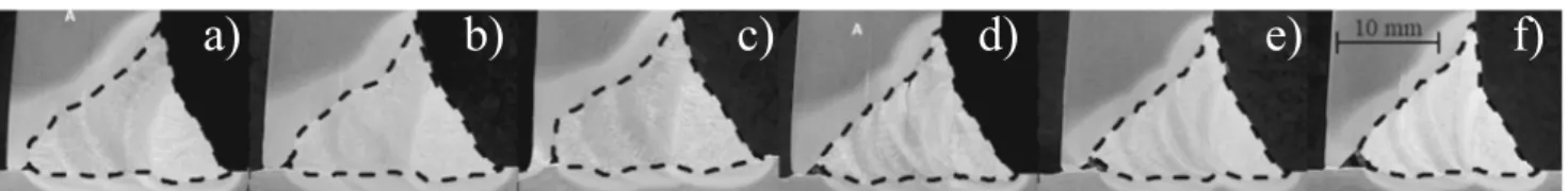
Fig. 8 Macrographs of single-bevel butt welds:a)–c) JT3-1-01–JT3-1-03 andd)–f) JT3-2-01–JT3-2-03

30 40 50 60 70 80 90 100

1.0 1.5 2.0 2.5

AFZ[mm2]

UI/v [kJ/mm]

Solid wire Flux cored

0 5 10 15

0 100 200 300 400 500

Ux,max[mm]

AFZ[mm²]

SBBW DBBW DSFW-S DSFW-M

a) b)

Fig. 9 Fusion zone size vs.a) maximum transverse deformations andb) total heat input per unit length

(12)

model. Solely solid wire electrodes are assumed in the calculations as the only aim of the sensitivity analysis is to evaluate the magnitude of differences in weld pool sizes, transverse deformations, and von Mises residual stresses.

The dimensions of T-joints with double-sided fillet weld are identical to the experimental ones, while throat thick- ness is 5 mm. A gap of 0.5 mm filled with“un-deposited material”is modeled between the base plate and the stiffener. The model consists of 27,010 finite elements (Fig.17). The minimum number of constraints is defined to analyze a statically determinate structure. Interpass temperature is not controlled, the second weld pass is laid right after the first weld pass with the same welding direction.

Welding variables areI= 270 A,Uis calculated using Eq.

(1), assuming solid wire electrodes, and v= 4 mm s⁻¹. Assuming flux cored electrodes in the calculation of voltage would only affect the heat input, while using different thermal efficiencies has the same effect. Ambient temperature is taken as 20 °C, while preheat temperature is 150 °C. The reference values for the characteristic parameters of Goldak’s double ellipsoidal heat source model are a=b=cf= 2.5 mm and cr= 4cf. These parameters are scaled in the sensitivity analysis to investigate the effect of power density distribution. Scaling factors of 1.00, 1.50, 2.00, 2.50, and 3.00 are applied; thermal efficiency is set to 1.00. Five additional analyses are performed in order to analyze the influence of thermal efficiency, which is in- creased in 0.10 steps from 0.60 to 1.00, while heat source

parameters are set to the reference values. Figures18,19, and20present the results of the sensitivity analysis.

Figure18shows weld pool size and isothermal lines in the vicinity of the weld in the midsection during welding of the first weld bead. Arrows show increasing tendency of fusion zone size. Scaling the reference heat source parameters results in lower power density. Thus, weld pool size decreases as scaling factor increases. Temperature does not even reach the liquidus temperature, assumed to be 1500 °C, in the weld bead elements when the scaling factor is equal to 3.00. The cross-sectional area of the weld pool is 47.5 mm², 45.5 mm², 36 mm², 12.5 mm², and 0 mm²using scaling factors of 1.00, 1.50, 2.00, 2.50, and 3.00, respectively. Variation of thermal efficiency has a similar effect as it has an influence on power density distribution; weld pool size increases as thermal efficiency increases. The cross-sectional area of the weld pool is 25 mm², 32 mm², 37 mm², 42.5 mm², and 47.5 mm²using thermal efficiency of 0.60, 0.70, 0.80, 0.90, and 1.00, respectively.

Figure 19 sums up the transverse deformations of the joint after cooling. Configurations a)–e) have maximum transverse deformations of 1.56 mm, 1.46 mm, 1.26 mm, 0.93 mm, and 0.45 mm, respectively. Transverse deformation of the stiffener decreases as scaling factor increases.

Arrows show increasing tendency of deformations. For instance, scaling factor of 2.00 results in a 20% decrease i n d e f o r m a t i o n s i n c o m p a r i s o n t o t h e r e f e r e n c e

0 50 100 150 200 250 300 350 400

0 200 400 600 800 1000

[ erutarepmeT°C]

Time [s]

Thermocouple

Infrared thermal camera Fig. 10 Temperature

measurements of a thermocouple and the calibrated infrared thermal camera

100 150 200 250 300 350 400

ss e n dr a H] V H[

Face1 Root1 Face2 Root2

BM HAZ FZ HAZ BM

a) b)

1 2

Fig. 11 a) Hardness profile for JT2-1-01 andb) points for measurements

(13)

configuration. Obviously, configurations d) and e) are er- roneous as temperature just reaches the reference temperatures in the finite elements representing the weld bead (Fig. 18), while the elevated temperature is lower than liquidus temperature in the corresponding finite elements.

Configurations f)–j) have maximum transverse deformations of 1.41 mm, 1.46 mm, 1.54 mm, 1.58 mm, and 1.56 mm, respectively. Transverse deformation of the stiffener slightly increases as thermal efficiency increases;

however, the variation is within 10% due to 67% increase in thermal efficiency.

Figure20shows the von Mises residual stresses in the vicinity of the weld beads in midsection after cooling. The plastic zones are shown in the figure, where the residual stress is higher than the yield strength, which is 355 MPa in this case. The same conclusions can be drawn as for

Fig.19. Arrows show increasing tendency of plastic zone size. Plastic zone size decreases as the weld pool size decreases. The signs of lack of fusion are presented for configuration e) for instance, where several finite elements in the weld bead remain elastic, while quasi-zero penetration is simulated in the joint.

Results show that thermal efficiency and the scaling factor may have a similar effect on residual stresses and transverse deformations. However, it is important to emphasize that sufficient power density is required to reach the reference temperature of un-deposited material; otherwise, the material model for weld bead elements remains elastic with a low Young’s modulus. It results in quasi-zero stresses in weld beads due to lack of fusion affecting overall residual stresses in conjunction with obtaining equilibrium of resultant internal forces and bending moments in any section of the specimen.

On the other hand, 100% increase in scaling factor for the first three cases results in a variation of 32% in the weld pool size, while the variation is within 90% due to 67% increase in thermal efficiency.

16 18 20 22 24 26 28 30 32

180 200 220 240 260 280 300 320

U [V]

I [A]

Solid wire electrode Flux cored electrode Fig. 12 Operating points and the

relationship between current and voltage for solid wire and flux cored electrodes

deformations strains stresses

temperature fields thermal gradients

HAZ and FZ determination

chemical composition phase proportions Vickers hardness

Mechanical problem

Microstructure Thermal problem

6 5

4 3

2 1

Fig. 13 Couplings in a thermo-metallurgical-mechanical analysis

Fig. 14 Notations and power density distribution of the double ellipsoidal heat source model

(14)

5.2 Evaluation of thermal efficiency

Generally, thermal efficiency of a welding process can be evaluated using several approaches. In the current study, it is determined by the comparison of experimental and numerical data. Thermocouples and infrared thermal imaging are utilized to carry out temperature measurements during welding, as presented in Section 3; thus, thermal cycles determined by finite element models can be compared with experimental data. In addition, macrographs are used to evaluate the thermal efficiency as well. Nevertheless, EN 1011-1:2009 [38] recom- mends to use 0.80 as thermal efficiency, while Radaj [27]

introduced a range between 0.65 and 0.90 for metal active gas welding. The sensitivity analysis in the previous section shows that thermal efficiency has a larger effect on fusion zone size than scaling the characteristic parameters of the heat source, while the latter has a negligible effect on total (elastic and thermal) strains and temperatures further from the weld bead as presented by Kollár and Kövesdi [8].

T-joints with double-sided fillet weld (JT2-1-06 and JT2- 2-02 welded with solid wire and flux cored electrodes, respectively) are chosen for the determination of thermal efficiency. The actual dimensions of the joints are modeled with the corresponding throat thicknesses. Throat thicknesses are

Fig. 16 Mechanical material properties based on EN 1993-1-2:2005 [35]

Fig. 15 Thermal material properties based on EN 1993-1- 2:2005 [35]