1. The shock front

VII. Shock wave structure in gases

§1. Introduction

The basic ideas on shock waves have been presented in Chapter I. It was shown that the hydrodynamic equations for an ideal fluid admit the existence of discontinuous solutions describing shock waves. The flow parameters, i.e., the density, pressure, and velocity on each side of the discontinuity sur- face, are connected by finite difference equations which correspond to the differential equations describing the continuous flow regions. Both the hydrodynamic and the difference equations are expressions of the general laws of conservation of mass, momentum, and energy. It follows from the conservation laws that the entropy of the fluid also undergoes a j u m p (in- creases) at the discontinuity surface. The increase in entropy across a shock wave is determined only by the conditions of conservation of mass, momen- tum, and energy and by the thermodynamic properties of the fluid, and is entirely independent of the dissipative mechanisms causing this increase.

It is somewhat paradoxical that the adiabatic equations of motion for a fluid admit the existence of surfaces where the entropy undergoes a jump. The irreversibility of a shock compression indicates the presence of dissipative processes, such as viscosity and heat conduction, which lead to the increase in the entropy. It is precisely the viscosity which results in the irreversible conversion into heat of a major part of the kinetic energy of the stream crossing the discontinuity, in a coordinate system in which the discontinuity is at rest. Thus, if we are interested in the mechanism of shock compression, in the internal structure and thickness of the transition layer in which the fluid is transformed from the initial to the final state and which, within the framework of the hydrodynamics of an ideal fluid, is replaced by a mathematical surface, we must turn to a theory which includes a description of the dissipative pro- cesses. In Chapter I this problem was considered for the case of weak shock waves. In this chapter we shall not impose any limitations on the strength of the shock.

Usually in hydrodynamic processes changes in the macroscopic parameters in regions of continuous flow occur very slowly in comparison with the rates of the relaxation processes which lead to the establishment of thermodynamic equilibrium. Each gas particle at any instant of time is in the state of thermo- dynamic equilibrium which corresponds to the slowly changing macroscopic variables, as though the particle " f o l l o w s " the changes in the variables.

465

Therefore, when considering shock discontinuities within the framework of the hydrodynamics of an ideal fluid, it is entirely permissible to assume the state of the gas on both sides of the discontinuity to be in equilibrium.

The density, pressure, etc. change very rapidly in the thin transition layer, through which the gas passes from its initial state of thermodynamic equi­

librium into its final, also equilibrium, state. The thermodynamic equilibrium inside this region, called here the shock front, can be appreciably disturbed.

Therefore, in studying the internal structure of a shock front it is necessary to consider the kinetics of relaxation processes and to investigate in detail the mechanism of the establishment of the final state of thermodynamic equilib­

rium in the fluid which is attained behind the shock front.

The study of the internal structure of shock fronts is of interest for many reasons. At first this problem attracted attention as purely a theoretical one, the solution of which aided in understanding the physical mechanism of shock compression, as a truly remarkable phenomenon in gasdynamics. Later shock waves were employed in laboratories with the aim of obtaining high tem­

peratures and of studying various processes which take place in gases at high temperatures, as for example, vibrational excitation in molecules, molecular dissociation, chemical reactions, ionization, and radiation (see Chapter IV).

Theoretical considerations of the shock front structure enable one to deduce from the experimental data a good deal of valuable information about the rates of these processes. Finally, the study of the structure of very strong shock fronts in which radiation plays an important role helps to clarify the problem of such an important characteristic as the luminosity of the shock front and makes it possible to explain some interesting optical effects observed in strong explosions in air (see Chapter IX).

The mathematical theory of shock front structure is based on the assump­

tion that the structure is steady. The time it takes the fluid in a shock wave to go from the initial to the final state is very short, much shorter than the characteristic times over which the flow variables change in the continuous flow region behind the shock front. In exactly the same way, the front thickness is much less than the characteristic length scale over which the state of the gas behind the front changes significantly, for example, the distance from the shock front to the piston " pushing" the wave (the piston moves with a nonuniform speed, in general). In the short time during which the shock wave traverses a distance of the order of the front thickness, its propa­

gation velocity, pressure, and the other flow variables behind the front remain practically unchanged. However, the kinetics of the internal processes which take place within a shock front propagating through a gas with given initial conditions depend only on the wave strength. Therefore over some relatively long period, each of the gas particles flowing into the shock discontinuity passes through the same sequence of states as the preceding ones. In other

§ 1 . Introduction 467

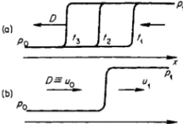
words, the distribution of the various variables across the shock front forms a " f r o z e n " picture which moves during this period as an entity together with the front (Fig. 7.1).

(a)

(b)

D=uⁿ

Fig. 7.1. Pressure distributions across a shock wave: (a) propagation of the shock in a laboratory coordinate system;

(b) the shock in a coordinate system moving with the front.

If we denote the front velocity by D (Z> = \D\ > 0), and the coordinate normal to the front surface at a given point by x, then we can say that all the state variables of the gas inside the wave depend on position and time only in the combination χ + Dt. In a coordinate system moving with the front the process is steady and is independent of time. This fact (which has already been used in deriving the relationships across the discontinuity) greatly simplifies the study of the problem from a mathematical point of view, since all the flow variables in the coordinate system moving with the wave are functions not of the two variables χ and i, but only of a single coordinate, and the process can be described by ordinary differential equations.

In considering the thickness of weak shock fronts in §23 of Chapter I, we have shown that the molecular mean free path serves as a characteristic scale of the shock thickness. As the wave strength increases, the thickness decreases, and when the increase in the pressure behind the front over the initial pressure becomes comparable with the initial pressure, the front thick­

ness is of the order of a molecular mean free path. It is physically clear that the thickness of a strong shock wave, where the compression takes place in the presence of " viscous " forces, is always of the order of a molecular mean free path*. This can be most simply explained by considering a shock wave in a coordinate system in which the gas behind the front is at rest (in a coordinate system moving with the piston) or, equivalently, by considering the bringing

* W e wish to emphasize the particular way in which w e use the concept of " viscosity "

in the case being considered. W h e n referring to viscosity, it is usually understood that the velocity gradients are small and that the velocity changes significantly only over distances much greater than a molecular mean free path. In other words, viscosity in hydrodynamics is a " m a c r o s c o p i c " concept. If a sharp change in gas velocity and density takes place over a distance o f the order of a mean free path, then this " microscopic" phenomenon may not be considered from the point of view of hydrodynamics but must be treated o n the basis of the kinetic theory of gases. A s applied to the case of very large gradients, the term

" viscosity " in the shock wave front denotes the mechanism by which the directed velocity of the molecules is changed to a random velocity by molecular collisions.

to rest of a high-velocity gas stream incident on a stationary wall. The kinetic energy of the directed molecular motion (the kinetic energy of hydro- dynamic motion) is converted into kinetic energy of random motion, i.e., into heat when the fluid is brought to rest. In order to " b r a k e " the fast molecules, whose directed velocity is much greater than the initial thermal velocity (in the case of a strong wave, with a hypersonic shock speed), several gaskinetic collisions are sufficient, since on the average each collision changes the direction of motion of a molecule through a large angle. Therefore, the directed momentum of the molecules is almost entirely scattered after several collisions and the velocities become random.

The distribution of energy over the various internal degrees of freedom, in particular vibrational excitation of the molecules, dissociation, and ionization, usually requires many collisions. The thickness of the relaxation layer in which the final thermodynamic equilibrium is established is much greater than the thickness of the initial shock wave. Hence the entire transition layer of the shock front can be divided into two regions with appreciably different thicknesses, a very thin " v i s c o u s " shock front and an extended relaxation layer.

In a sufficiently strong shock front in which the gas is heated to high temperatures, an important role is played by radiation and radiative heat transfer. The structure of the front in this case becomes even more complex.

The total front thickness is determined by the largest scale characterizing the transition process associated with radiant heat exchange, namely the radia- tion mean free path, which ordinarily is many times greater than the gas- kinetic mean free path.

In the following sections we shall consider in detail the characteristic properties of the structure of shock fronts. We start by considering relatively weak shock waves, after which we shall consider increasingly stronger waves.

1. The shock front

§2. Viscous shock front

Since the compression shock in a shock front takes place over distances comparable with the gaskinetic mean free path, we should actually begin our study of shock front structure on the basis of the kinetic theory of gases. As a first step in this direction, however, it is natural to consider the problem in the framework of the hydrodynamics of a real fluid, in which dissipative processes are taken into account, i.e., with viscosity and heat conduction. Here, in contrast to §23 of Chapter I, we do not impose any limitations on the strength

§2. Viscous shock front 469

of the shock wave. To provide continuity of presentation we repeat here some conclusions and calculations of that section. In order not to complicate the presentation by unnecessary detail connected with the slow excitation of nontranslational degrees of freedom, we regard the gas as monatomic and neglect ionization.

The one-dimensional flow equations for a viscous and heat conducting gas flow which is steady in a coordinate system moving with the wave front are

d

— p^W = o, dx

du ^dp d 4 du ^ ^ ^

^^U dx dx dx 3 ^ dx puT — --μ(—dx 3 \dx) dx

Y- —

Here Σ is the specific entropy*, μ the coefficient of viscosity!, and S is a

* Editors' note. T h e reader is cautioned to n o t e that the symbol S used elsewhere in the book to denote specific entropy is going to be consistently used for energy flux, particularly for radiant energy flux, and therefore a new symbol had to be used for entropy in this chapter.

t For the case considered the concepts of first and second viscosities are indistin­

guishable.

Editors' note. More specifically, their effects are combined into a single term. A s in the analysis of §23, Chapter I, we may include second or bulk viscosity by replacing f/x by the longitudinal coefficient μ" = f μ + μ'.

Dilute monatomic gases have μ' = 0, and the usual physical origin of bulk viscosity is in rotational relaxation. A s discussed in §2 of Chapter VI, the rotational relaxation time

rr o t is extremely short, though it may be appreciably larger than the characteristic transla-

tional or gaskinetic collision time of (6.1), Chapter VI.

On the assumptions that rTOt is large compared with rg a s but small compared with a characteristic macroscopic time scale, and that vibrational m o d e s are unexcited, a relation between μ' and rr o t may be established. T h e quantity p of (1.95), Chapter I, is given by p = pRTtrans, while pst is given by pst = ρ(γ — \)(ctT!insTtrans + cr o t7r ot ) , with ct r a n s + crot = c and ( y — l)c„ = R. Thus we identify

, Dp cr o t

ρ — pst = μ —zr- = pR{TUans — Trot) — ·

put cv

With τΓο ι > T tr an s and the rotational m o d e governed by a relaxation law, we have DTTOt

TtTans TTot Dt ~ T r o t

Finally, with Tr ot small in comparison with the macroscopic time scale, we may approximate DTroi DTtrtns j t y ( y - l )2g Dp

~ΈΓ^~5Γ^^{ΚΎ l)ltTans}pDt™ R pDt'

nonhydrodynamic energy flux, equal according t o the ordinary heat con­

duction law t o

S = - K ^ \ (7.2)

ax

where κ is the coefficient of thermal conductivity. To the system of equations (7.1) must be added the boundary conditions expressing the absence of any gradients ahead of and behind the wave front, and also the fact that the flow variables must approach their initial (for χ = — oo) and final (for χ = + oo) values.

Rewriting the third equation in (7.1) by means of the relation Τ dl = de + ρ dV = dh - - dp

Ρ

and integrating each equation in (7.1), we obtain the first integrals of the system

pu = p⁰D,

ι 4 du ~

p + p u

_ _

_

, u² 1 / 4 du\ , D²

The constants of integration are expressed here in terms of the initial values of the flow variables, distinguished by the subscript " 0 " and by the front velocity D = u⁰.

If we refer the system (7.3) to the final state (denoted by the subscript "1")

Eliminating Τ^ίΓΛη* — T^rot and Dp/Dt yields the result

μ' = (γ- Ό2ρε— Tr o t. c^v See Kohler [100].

If r^{r o t} is not much larger than T^{g a s}, the relaxation analysis above does not apply. The relation above then may be considered t o indicate correct orders o f magnitude. For either diatomic or polyatomic molecules,

£ - 0.1632L.

μ r^{g a s}

The quantity Tr o t is the relaxation time for a process in which TitaM is kept fixed. For a process in which ε = c^{t r}ans7trans + c^rotT^tot is kept fixed, the relaxation time is c^transT^totlc⁰. The distinction between these two definitions o f the relaxation time should be kept in mind.

§2. Viscous shock front 471

we obtain the already well-known relations across a discontinuity, which we repeat here for convenience

P i " i = Po^D>

Pi + Ρ ι " ί = Po + PoD², ^ ^

It follows from these equations that the entropy j u m p across a shock wave Σ1 — Σ0 = Σ(ρΐ9 ρ χ) — Σ(ρ0, ρ0) is entirely independent of both the dissipative mechanisms involved, or in this case of the values of the coefficients of viscosity and thermal conductivity μ and κ. The latter determine only the internal structure of the wave front and its thickness δ. The thickness δ of the viscous shock front is proportional to the coefficients μ and κ, which in turn are proportional to the molecular mean free path /. In the limit / -> 0 the hydrodynamics of a real fluid becomes, in the continuous flow regions, the hydrodynamics of an ideal fluid. The shock front in the limit / 0 becomes a mathematical surface, since δ ~ I 0. In this case, the gradients of all the flow variables across the front tend to infinity as 1 // but their jumps remain finite.

Specifying the coefficients of viscosity and thermal conductivity and also the thermodynamic relation h(p, p) (in a monatomic gas h = c^pT = \p\p), we can numerically integrate the system (7.3) and (7.2) with the given boundary conditions. However, it is much more convenient to have an analytic solution, since it illustrates graphically all the relationships governing the phenomenon.

Unfortunately, it is not possible in general to find an analytic solution to the system. The equations can be integrated analytically if we limit ourselves to weak waves and expand the solution in a series with respect to the small change in one of the flow variables. This method was used in §23 of Chapter I for estimating the front thickness (the complete solution is given in the book by Landau and Lifshitz [1]). An exact analytic solution for a wave of arbitrary strength can be found in one special case. This solution, first obtained by Becker [2] and subsequently investigated by Morduchow and Libby [3], describes all of the physical laws governing the structure of a shock front, and is both simple and graphic. Let us describe this solution in more detail.

Usually the transport coefficients in gases, that is, the values of the kine­

matic viscosity ν = μ\ρ and of the thermal diffusivity χ = K/c^pp, are close to each other and to the diffusion coefficient Ινβ. Let us set the dimensionless group Pr = pcpJK = ν/χ, called the Prandtl number, equal to 3/4. In this case the expression in parentheses in the last of equations (7.3) becomes a total

differential of the quantity h + w²/2, and the equation becomes u²\ 4 μ d / u²\ ^f D²

h +

V -3^T

{

+V=

»

T-

In writing the integral of this linear equation, it is evident that h + w²/2 can be finite at χ = + oo only if it is independent of x,

u² D² *

ft+- = ft⁰+— . (7.5)

Thus, for a Prandtl number equal to 3/4, (7.5) is satisfied not only behind the shock front (see (7.4)), but also at any intermediate point x.

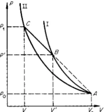
Equation (7.5) gives a curve in the /?, V plane along which the gas changes from the initial to the final state. Noting that for the monatomic gas under consideration h = %pV, and introducing the dimensionless velocity or specific volume

_^__X_ ⁼ Po

η ~ D ~ V⁰ " ρ ' we find the equation of this curve is

ρ 1 + ^ Μ²( 1 - η²) Αη, - η²

(7.6)

= ~Λ ~Λ ~ ΪΛ2 ⁼ Τ Τ ΤΤι ' (⁷·⁷) Po f (4>?ι - 1)η

Here ^! refers to the final state behind the shock front 1 , 5 _ P o _ _ 1 3_L

4 p⁰D² ~4 ⁺ 4M

and A / is the Mach number Μ = Djc⁰, where c⁰ is the speed of sound in the initial state (cq = | p⁰^ o ) - Iⁿ deriving (7.6) and (7.7) we have made use of the equations relating the variables on both sides of the shock front. The Hugoniot equation in terms of the variables Pilp⁰ and η^ί is

Pi 4 - ^ Po 4^ηι - 1

Figure 7.2 shows the Hugoniot curve and the curve along which the state of a particle changes through the wave (and also the characteristic straight line connecting the initial and the final states).

Using (7.6) and the first two equations of (7.3), let us write a differential equation describing the velocity and specific volume distributions through

* This equation is analogous to the Bernoulli equation in steady flow theory.

§2. Viscous shock front 473

the shock front η(χ)

5 Ρ ^dr1 η ν \ (7.8)

For simplicity, the coefficient of viscosity is assumed to be independent of temperature and equal to μ = ρ⁰1⁰ν⁰β (it is independent of density, since

Fig. 7.2. Shock transition A-^B ona.

ρ, V diagram. Η is the Hugoniot curve.

The point describing the state inside the wave front passes from A to Β along the dashed line.

μ ~ pi, and I ~ 1/p). The integral of (7.8) contains an additive constant con­

sistent with the arbitrariness in the choice of the coordinate origin. Locating the origin at the point of inflection of the velocity profile (in the " center "

of the wave) and using (7.7), we find for η(χ) the expression

in-ηιΤ (y/^-^r L μ ι⁰] ν 40 V 6 / (7.9) Knowing the velocity profile u = Βη, it is easy to determine the distribu­

tions of the other variables. Thus, for the temperature we have from (7.5) TjT⁰ = 1 + \M²{\ — η²); the pressure is defined in terms of η by (7.6) and the entropy is

Σ - Σ⁰ = c^p In J - R In — (R = -^).

P T⁰ Ρο \ PTJ

It is evident from (7.9) that as χ -> — oo, η 1 and as χ -> + oo, η -> η^ί9 with the initial and final values being approached asymptotically in an expo­

nential manner. All the flow variables velocity, density, pressure, and tem­

perature change monotonieally across the wave from their initial to the final values, which are approached asymptotically as χ ^ Τ oo*. The entropy, on the other hand, does not change monotonieally, and has a maximum within the wave (this has already been shown in §23, Chapter I). We can easily satisfy

* The inflection points for the various variables in the wave front do not coincide.

ourselves that this is so by rewriting the entropy equation (the third of equa­

tions (7.1)) with the aid of the second law, the "Bernoulli e q u a t i o n " (7.5), and the second of equations (7.1). We find

άΣ (dh dp\ ( du d 4 du du\

puT — = pu[ — - V — ) = pul -u — -V — -p—+Vpu — \ dx \dx dxj \ dx dx 3 dx dxJ

d 4 du u

U dx 3 ^ dx 3 ^ dx²

It is evident that the entropy has an extremum at the inflection point in the velocity, that is, at the wave " c e n t e r " . The existence of an entropy maxi­

mum in the wave is connected with the presence of heat conduction. One of the dissipative processes, viscosity, produces only an entropy increase, proportional to {dujdx)². Heat conduction, however, produces an irrevers­

ible transfer of heat from the hotter to colder gas layers. Here the increase in entropy of fluid particles through heat conduction in the colder layers (where dSjdx ~ —d²Tjdx² < 0) is positive, and in the hotter layers (where dSjdx d²T/dx²>0) is negative.

The entropy decrease in the more heated layers does not in any way con­

tradict the second law. The entropy of the gas as a whole or of an individual particle increases across the whole shock discontinuity as a result of the process of shock compression. However, an individual layer of gas passing through the wave is no longer an isolated system. Its entropy increases at the beginning, when it is supplied heat through heat conduction and the work of the viscous forces, and then decreases when the heat loss due to heat con­

duction in the direction of the colder gas layers behind it exceeds the heat supplied by the work of the viscous forces.

The front thickness, as in §23 of Chapter I, is given by

3=- ^D ~ ^U i

(du/dx)^max

It is evident from (7.9) that the order of magnitude of the front thickness is Μ

δ~ 1⁰ Μ² - 1

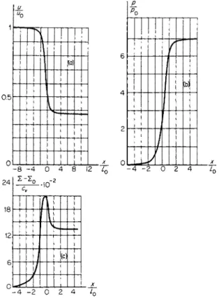
In a weak shock wave when Μ — 1 <^ 1, δ ~ l⁰l(M — 1), in agreement with the results presented in §23 of Chapter 1. In this case, the front thickness can be equal to many molecular free paths. In the case when Μ = 2, shown in Fig.

7.3, the front thickness is approximately equal to three molecular free paths /⁰. In the limiting case of a strong wave, when Μ -> oo, δ ~ /⁰/Λ/->0. The statement that the front thickness vanishes as the wave strength increases

§2. Viscous shock front 4 7 5

should, of course, not be taken literally*. The fact is simply that when the front thickness becomes of the order of a mean free path, the hydrodynamic theory loses its meaning, since it is based on the assumption that the gradients are small, that the mean free path is small in comparison with the distance over which appreciable changes in the flow variables take place. Hence the theory

0. 5

(a)

I

>

- 8 - 4 0 4 8 12 U

(b)

J

4 - 2 0 2 4 L

2 4

18

Σ -Σ,

-°-.ιο"²

I

I

(0

>

/

- 2 0 2 4

Fig. 7.3. Distributions of (a) velocity, (b) pressure, and (c) entropy through a viscous shock front with Mach number Μ = 2 in a gas with a specific heat ratio y = 7/5 and a temperature-independent viscosity coefficient. The abscissa is in units of molecular mean free path in the undisturbed gas (the graphs were taken from [3]).

* Editors' note. The result that δ ~ Io/M^0 as oo is somewhat artificial. It is based on the assumption that μ is constant through the wave. Since μ ~ pvl and p⁰/ p i ~ 1, vl remains of the same order through the wave. But ϋ^ν ~ Mv⁰, and Ιι ~ /⁰/ M - > 0 as M - > oo if /⁰ is kept fixed. But δ ~ h in the same limit, and δ remains finite if Λ does.

The conclusion δ ~ l^u that the shock front thickness is of the order of a few mean free paths in the flow behind the shock, is a general one for strong shocks. Even though the Navier-Stokes equations are invalid for strong shocks, they nevertheless give not only correct order-of-magnitude results, but also quite faithful numerical results for the macro­

scopic flow variables except in the upstream part of the shock front.

is simply inapplicable for sufficiently strong waves. It is evident physically that the thickness of the shock front for a wave of any strength cannot become smaller than the mean free path, since the gas molecules flowing into the discontinuity must make at least several collisions in order to scatter the directed momentum and to convert the kinetic energy of the directed motion into the kinetic energy of random motion (into heat). At the same time, the thickness of the shock front in the case of a strong wave cannot include many mean free paths, since the molecules of the incident stream lose, on the average, an appreciable fraction of their momentum during each collision.

The problem of the structure of strong shock fronts must be treated on the basis of the kinetic theory of gases, and hence the many numerical studies concerned with the improvement of the simple theory presented above, by taking the dependence of the transport coefficients on temperature into account, by calculating the effect of the Prandtl number on the front structure, and so forth [4-13], do not contribute anything new in principle beyond the particular case considered above, and at best are of interest for the case of weak waves only*.

Tamm [101], and independently Mott-Smith [16], applied the Boltzmann kinetic equation to the problem of the structure of a shock front. An approxi­

mate solution to the Boltzmann equation in the neighborhood of the shock front is constructed as a superposition of two Maxwellian distributions corresponding to the temperature and macroscopic velocity in the initial and final states. The relative weight of each function varies over the width of the wave from 0 to 1. The front thickness for an infinite strength shock wave tends to a finite limit. Sakurai [17], who has somewhat refined Mott-Smith's method on the basis of a hard-sphere model for the molecular interactions, obtained shock thicknesses in units of mean free path based on the initial conditions, of f S/l⁰ = 2.11, 1.68,1.46, and 1.42 for Mach numbers of Μ = 2.5, 4, 10, and oo, respectively. We note several other papers which have developed

* A n attempt to refine the hydrodynamic approximation by taking into account second derivatives in the expressions for the transfer terms (the so-called Burnett approximation), undertaken by Zoller [14], somewhat improves the results for weak waves and, essentially, only points out the limits of applicability of the hydrodynamic theory. For a wave strength PilPo = 1.5, the thickness of the front, according to Zoller, is equal to 17 mean free paths, and for pjpo = 4 is equal to 6 mean free paths. The front thickness of weak shock waves in monatomic gases was measured by Greene, Cowan, and Hornig [15] using a method based on the reflection of light (see §5 of Chapter IV). The thickness was found equal to 30, 19, and 13 mean free paths for Mach numbers Μ = 1.1, 1.5, and 2.5, respectively. Zoller's calculations are in not t o o bad agreement with these results. See also [56].

t The front thickness δ is defined in the following manner. If fa and fp are the molecular distribution functions in the initial and final states, then the distribution function at an intermediate point χ in the wave is, according to the theory, / = ν(—χ)/^Λ-\- v(x)f^p, where v(x) = 1(1 + tanh(2*/8)).

§3. Viscosity and heat conduction in shock front formation 477

Mott-Smith's method and treated the shock front on the basis of the Boltz­

mann equation [52-55].

§3. The role of viscosity and heat conduction in the formation of a shock front Despite the fact that the values of the transport coefficients—kinematic viscosity and thermal difTusivity, or the corresponding dissipative terms in the energy equation—are close to each other, the contribution of each of these dissipative processes to the formation of a shock are far from equal. Physi­

cally, it is clear that the principal role in the mechanism of shock com­

pression is played by viscosity rather than heat conduction, since it is the viscous mechanism which causes the scattering of the directed momentum of the incident gas and the conversion of the kinetic energy of the directed molecular motion into the kinetic energy of random motion, i.e., the con­

version of mechanical energy into heat. Heat conduction, on the other hand, only indirectly affects the conversion of mechanical energy as a result of the redistribution of pressure. In order to satisfy ourselves of this, it is useful to consider the problem of a one-dimensional steady flow of a gas through a shock front under the assumption that viscosity is completely absent and that the dissipation is caused by heat conduction only. An investigation of this problem (first carried out by Rayleigh [18]) is of considerable interest, since it illustrates the features of the structure of a shock front in the presence of other mechanisms of heat exchange, e.g., radiative heat transfer or electron heat conduction (in a plasma).

By neglecting viscosity, the first integrals in the hydrodynamic equations for one-dimensional steady flow (7.3) take the form

It follows from the first two equations of (7.10) that in the process of shock compression, in the absence of viscosity, the state of a gas particle must change continuously along a straight line in the pressure-specific volume diagram

ρ + pu² pu

Po + PoD², (7.10)

ρ = Po + P o ^²( i -1 ) , V

(7.11) This important property of inviscid gas flow is illustrated in Fig. 7.4, which shows a Hugoniot curve and a straight line connecting the initial and final states of the gas.

We shall attempt to solve the system of equations (7.10) where, as before, we shall eliminate all variables except the dimensionless velocity or relative specific volume η. For generality, we shall not restrict our problem to a

Fig. 7.4. Straight line shock transition for an inviscid gas.

monatomic gas and shall retain an arbitrary constant specific heat ratio.

Noting the equation of state

p = — pT = RpT, R = — (7.12) (μ⁰ is the molecular weight), and the thermodynamic relation h =

[yl(y — 0 ] WP »^{w e} express by means of the third equation of (7.10) and (7.11) the nonhydrodynamic energy flux and temperature in terms of η,

L

2

_^__i_y

s = - ^ — A i - v X n - n d - (7.14) 2 y — 1

Here, as before, the quantity

7 - 1 2 1 y + l 7 + 1 Μ

is the dimensionless velocity in the final state and Μ = D/c⁰ is the Mach number.

The function Τ(η) passes through a maximum at the point _ 1 1

η~^η™^χ~2*2ΪΜ²~'

Two cases can be encountered in considering shock waves of different strengths. If the shock is sufficiently weak, then η^ί > ^y^{m a x}. Indeed, for a Mach number close to unity (M — 1 <^ 1), we find η^ί « 1 — [4/(7 + \)]{M — 1), so that it is also close to unity, while J7^{M A X} « (7 + \)/2y < 1. In this case, a monotonic compression of the gas from the initial to the final volume (from η = 1 to η = η^χ) results in a monotonic increase in the temperature from the

§3. Viscosity and heat conduction in shock front formation 479

initial value T⁰ to the final value Γ,, given (under the assumed conditions) by

J

?<iz±V_,/

0 - • (y + D^{! v} Λ ίΜ',

The curves of Τ(η) and Ξ(η) in this case have the shape illustrated in Fig. 7.5.

1 [_ χ \ Fig. 7.5. Τ,η and 5 , ^ diagrams for

the case when a continuous shock tran-

^ 1 sition with heat conduction only is pos-

" sible, without considering viscosity.

Fig. 7.6. Temperature and entropy distributions in a shock wave with heat conduction only (without viscosity) in the case when a continuous transition is possible.

By eliminating η from (7.13) and (7.14) and substituting (7.2) for S, we obtain a differential equation of the type dTjdx = f (T) which has a con­

tinuous solution. The temperature and entropy distributions in such a wave are represented schematically in Fig. 7.6. They are quite similar to the distributions found in the preceding section. It is evident from the entropy equation (7.1) with μ = 0, that the entropy has a maximum at the point where d(x dT\dx)\dx = 0, or in the case of κ = const where the temperature in the wave T(x) has an inflection point, i.e., where d²T/dx² = 0. Therefore, a weak shock wave with a continuous distribution of flow variables across the front can also exist in the absence of viscosity, with only heat conduction present.

Let us now consider a sufficiently strong shock wave. In this case the specific volume for which the temperature assumes its maximum value lies between the initial and final values: η^χ < ^y^{m a x} < 1. Actually, for M > 1,

*/max ^ 1/2, and η^γ = (y — l)/(y + 1) < 1/4, since the specific heat ratio

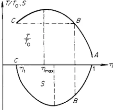
cannot exceed 5/3. Thus, for a continuous monotonic compression of the gas from its initial to its final volume, the temperature across the wave front must necessarily pass through a maximum. Plots of the functions Τ(η) and Ξ(η) for this case are given in Fig. 7.7. Let us investigate the possibility of the existence of a continuous solution of (7.13) and (7.14) in this case. It

can be seen from (7.14) and Fig. 7.7 that the heat flux S caused by heat conduction does not change sign over the entire range in which the relative volume changes from η = 1 to η = η^χ and it is opposite to the direction of gas flow, i.e., S < 0. In accordance with the definition of the flux S =

— κ dTjdx, the temperature can only increase as the volume changes from its

initial to its final value: dT/dx>0. Consequently, the region behind the temperature maximum, where dT\dr\ > 0, is not realized. In this region the specific volume has not yet reached its final value and must decrease, with dr\\dx < 0; the temperature, however, also decreases with decreasing volume, with

and the heat flux would have to be directed in the opposite direction (S > 0), in contradiction to (7.14).

Thus, a continuous distribution of temperature and density with respect to position is impossible in the case of a strong wave in which only heat con-

Fig. 7.7. Τ,η and δ,η diagrams for the case of an isothermal jump, taking into account heat conduction alone but without taking viscosity into account.

dT _ dT άη dx άη dx

Fig. 7 . 8 . Temperature and density pro­

files in a shock wave with an isothermal jump.

Ο ^χ

Pi

0 χ

duction is taken into account. Starting from the initial state, the final state can be reached without passing through the temperature drop region caused by the increased compression only if a discontinuity is allowed in the solution.

§3. Viscosity and heat conduction in shock front formation 481

In particular, there is a continuous change from the initial state (point A on Fig. 7.7) to point B, and then there is a jump to the final point C. The formation of a density j u m p indicates that viscous forces must be present, and that a strong discontinuity can disappear only through the action of viscosity but not of heat conduction. The temperature in the jump remains constant, and only its derivative, i.e., the flux, changes. The temperature and density profiles in such a wave, which is called an " i s o t h e r m a l " shock, are shown in Fig. 7.8*.

It is easy to find the largest strength for which a continuous solution in the absence of viscosity is still possible. This strength corresponds to the case in which the maximum of the function Τ(η) coincides with the final state, when *7^{m a x} = η^ι. In this case, the Mach number and the pressure ratio across the front are given by

M , ^{= /} 3 y - l γ /² pi + l y(3 - i)J Po 3 - γ

For example, for y = 5/3, M' = 1 . 3 5 and p[/p⁰ = 2, while for y = 7/5, M' = 1.2 and/>;//><>= 1.5.

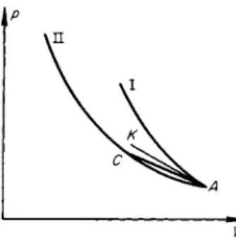
If we consider the other limiting case, when there is only viscosity and heat conduction is absent, we obtain a continuous solution for the flow variables across the shock wave which does not differ basically from the solution of the preceding section, with the single exception that the entropy in this case also increases monotonieally (see the third equation of (7.1) without the term dSjdx). The behavior of the entropy in both limiting cases can be clarified by considering a/?, V or a ρ, η diagram (Fig. 7.9). In the absence of viscosity

Fig. 7.9. />, V diagram for a shock wave, taking viscosity into account.

His the Hugoniot curve; Σ⁰, Σ^{ΐ 5} and Σ' are isentropes; the transition from the initial to the final state takes place along the dashed curve.

the state in the wave changes along the straight line A Β and the entropy (as is evident from a comparison of the Hugoniot curve with the isentropes) first

* W e note that the ^{4 4}i s o t h e r m a l " character of the shock, i.e., the continuity of tempera­

ture across the shock front, is a consequence of the assumption that the heat flux is pro­

portional to the temperature gradient. In the third part of this chapter, in considering radiant heat exchange in a shock front, we shall see that without this assumption the temperature will also have a discontinuity.

increases, reaching a maximum at the point of tangency of the straight line and the isentrope Σ', and then decreases. In the absence of heat conduction the state changes along the dashed curve which passes below the straight line A Β (the equation of this curve is ρ = p⁰ + PoD²{\ — η) + f p du/dx, where dufdx < 0), and it is nowhere tangent to the isentropes. The situation here is completely analogous to that which exists in the weak waves con­

sidered in §23 of Chapter I.

§4. Diffusion in a binary gas mixture

The presence of gradients in the thermodynamic quantities of a gas mixture gives rise to diffusional fluxes in the components of the mixture, which results in a redistribution of their concentrations. In general, diffusion tends to equalize the spatial concentrations of the components. However, the existence of pressure and temperature gradients or of an external force field such as gravity, centrifugal forces in rotating mixtures, or the presence of an acceler­

ation results in component separation in an initially homogeneous mixture.

In particular, such a situation arises in a shock wave propagating through a gas mixture. The concentrations of the components behind and ahead of the front are uniform and constant in space. In the region of the front, where gradients are present, these concentrations change. As with viscosity and heat conduction, diffusion represents an irreversible molecular mass transfer of a specific component (viscosity is responsible for momentum transfer and heat conduction for internal energy transfer) and is one of the sources for the dissipation of mechanical energy.

The diffusional flux is defined as follows. Let the mass concentration of one of the components in a binary gas mixture, for example, of the light component whose molecular mass is m^u be equal to a. The concentration of the second, heavy component whose molecular mass is m²{rn²> rn^x) is

1 — a*. As a result of the diffusion of one gas with respect to the other the gases have different macroscopic velocities, which we denote by u^t and u². If ρ is the density of the mixture, then the total flux of the first component is pauj, and the flux of the second component is p(l — a ) u². The macroscopic or hydrodynamic velocity of the mixture u is defined in such a way that the total mass flux of the gas is equal to pu (u is the momentum per unit mass). Thus, pu = pau¹ + p(l — a)u² or u = au, + (1 — a)u² . Within the framework of the

* The mass concentration α is equal to the mass of the first, light component, per unit mass of the mixture. If the number of molecules per unit mass of mixture is Ni and N² (Ni + N² = N)⁹ then α = JVi/Wi and 1 — α = N2m² . The molar concentrations are

Μ _ _ α _ Ν² _ 1 - α Ν Nnii ' ~Ν ~ Nm² '

§4. Diffusion in a binary gas mixture 483

hydrodynamics of an ideal fluid (without diffusion), the velocities of both components of the mixture are the same and equal to u. The fluxes of the components are equal to pau and p(l — a)u.

In the next approximation there appear in the hydrodynamic theory vis­

cosity, heat conduction, and diffusion (in the mixture). The diffusional flux i refers to the difference between the total and the hydrodynamic fluxes of one component, say the first component, i = pau^l — pau = ρ α ( ^ — u). The total flux of the first component is equal to the sum of the hydrodynamic and diffusional fluxes pau + i. The total flux of the second component is, obviously, p(l — a)u² = p(l — a)u + p(l — a)(u² — u) = p(l — a)u — i. The diffusional fluxes of the two components in a binary mixture are of the same magnitude but of opposite direction.

As pointed out above, diffusion arises as a result of the presence of con­

centration, pressure, and temperature gradients in a gas*. In the one-dimen­

sional case the gradients are simply equal to derivatives with respect to x, and the vector i has only an χ component which will be denoted simply by /.

The diffusional flux is given by (see [1])

Here D is the diffusion coefficient, k^pD is the pressure diffusion coefficient, and k^TD is the thermal diffusion coefficient. The dimensionless quantity k^p is determined only by the thermodynamic properties of the mixture and is given by (see [l]t)

For m²> m^u k^p> 0 and the pressure diffusional flux of the light component is in the direction of decreasing concentration. The flux caused by the con­

centration gradient is also in the direction of decreasing concentration (for either component). The thermal diffusional flux of the light component for

* The state of a binary mixture is characterized by three thermodynamic variables: the concentration and any two of the usual variables such as temperature, pressure, and density.

In studying diffusion, it is convenient to choose pressure and temperature as the independent variables.

t In the absence of viscous m o m e n t u m transfer (see below).

% The quantity k^p is most simply derived by considering an equilibrium binary mixture in a gravity field at constant temperature. In equilibrium the molecular number densities rii and η², from the Boltzmann equation, are expressed in proportional form as η ~ exp(—migx/kT\ and n² ~ exp(—m²gx/kT\ where g is the acceleration of gravity and Λ: is the altitude. Since the equilibrium diffusional flux is equal to zero, doc/dx + (k^p/p) dp/dx = 0.

Using the relationship between the concentration α and the particle number densities Wi and n2 and noting that p = (n1+ n2)kTy we find the above equation for kp.

(7.15)

(7.16)

most mixtures is in the direction of increasing temperature (for m²>

k^T < 0).

In contrast to k^p, the thermal diffusion ratio k^T depends not only on the component concentrations (for α = 0 or 1, k^T = 0) and the molecular masses, but also on the law governing the molecular interactions. The quantity k^p is determined purely by the thermodynamic properties of the gas, since thermo­

dynamic equilibrium is possible even in the presence of a pressure gradient in an external force field. If a temperature gradient is also present, then the gas is no longer in a state of equilibrium. If only repulsive forces varying as 1/r" are acting between the molecules, then for η > 5, which is usually the case, k^T < 0: the light gas will diffuse in the direction of increasing tempera­

ture. For η < 5, which is rarely encountered, the light gas diffuses in the direction of decreasing temperature (the case of η < 5 includes the Coulomb law for the interaction of charged particles, for which η = 2). When η = 5 thermal diffusion is absent and k^T = 0. Usually, when the relative gradients Vp/p and \T/T are comparable, the importance of thermal diffusion is small in comparison with pressure diffusion. For further details on thermal diffu­

sion see [19]. With the diffusional flux is connected an additional irreversible energy flux q, which is proportional to the diffusional flux i (see [1]).

Zhdanov, Kagan, and Sazykin [19a] have introduced an important cor­

rection to the classical diffusion concepts presented above. These authors derived an expression for the diffusional flux from the kinetic equation, using the Grad "thirteen m o m e n t " method. This method of approximation has a number of advantages over the Chapman-Enskog method used to obtain (7.15), whenever it is necessary to take into account higher approximations in the expansion of the distribution function. It is found that equation (7.15) for the diffusional flux is valid only in the absence of viscous momentum transfer in the gas. Under conditions when viscous momentum transfer is present (that is, when there is a velocity gradient) equation (7.15) must also include terms proportional to the viscous forces. In spite of the fact that these forces are determined by second-order derivatives of macroscopic quantities (such as velocity), they can be of the same order as terms proportional to first-order derivatives such as the term with pressure gradient. For example, in the case of a purely viscous steady flow without acceleration, the pressure gradient is simply balanced by the viscous forces. In the case of unsteady flow, the inclusion of viscous forces in the expression for the diffusional flux actually introduces into this expression terms proportional to the acceler­

ations of the gas.

In the case of purely viscous flow, the replacement of the viscous force by the pressure gradient which balances it results in a change in the pressure diffusion constant k^p in comparison with its purely thermodynamic value (7.16). The pressure diffusion constant is no longer a thermodynamic quantity

§5. Shock wave in a binary mixture 485

in a viscous flow; it depends on the character of the molecular interaction.

The pressure diffusion constant under some conditions can become negative (in the case when the molecular weights of the components differ very slightly from each other and when the molecular cross sections are appreciably different). When viscous momentum transfer is taken into account, the ther­

mal diffusion ratio k^T also changes.

§5. Diffusion in a shock wave propagating through a binary mixture

Let us consider what happens when a shock wave is propagated through a binary gas mixture. Large gradients in the thermodynamic quantities are present in the shock front and, as a result, conditions for diffusion are favorable. Physically, it is clear that the light component will concentrate in the shock front. Indeed, in the heated gas behind the shock front the mol­

ecules of the light component have a higher thermal velocity than the molecules of the heavy component (ν ~ (T/m)^1/2). Therefore, the light molecules " p u l l a h e a d " and leave the heavy molecules slightly behind (in the laboratory coordinate system, where the original mixture is at rest).

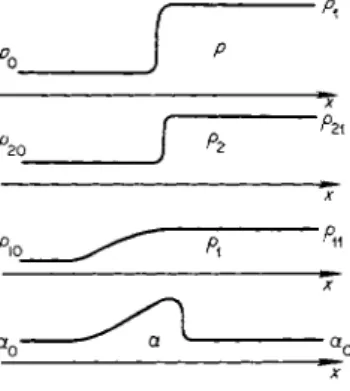
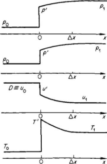
Let the heavy gas have a small admixture of the light gas. Then the density distributions of both the heavy and light gases ( p² and p^x) in a strong shock wave have the form shown in Fig. 7.10. This figure also shows the concentra­

tion distribution of the light component α = Ρι/(ρ² + Pi)- The thickness of the

Fig. 7.10. Pressure and density dis­

tributions of the heavy ( p²) and light (pi) components and concentration of the light component (a) in a shock wave propagating through a binary gas mixture.

region containing the higher concentration of the light component is of the order of Ax ~ Dju⁰, where D is the diffusion coefficient and u⁰ here denotes the shock velocity*. The diffusion coefficient D is of the order of Ιϋ^ί9 where

* This follows from the condition that the total flux of the light component is steady in a coordinate system moving with the front. Approximately p\U^Q = D dpi/dx, from which pi = pi ι e x p ( —u⁰ \x\ ID). Here we have used an approximate boundary condition according to which we can assume that the density of the light component at the point χ = 0, where the viscous shock front is located, is equal to its final value pu.

is the thermal speed of the light gas heated by the shock wave and / is the molecular mean free path. The velocity of the front u⁰ is of the order of the thermal speed of the heated heavy gas, u⁰ ~ v². But v^xjv² « ( m²/ m¹)^{1 / 2}, so that Ax « ( m²/ m¹)^{1 / 2}/ . The thickness of the viscous shock front is of the order of /. Consequently, the thickness of the region in which the light component is concentrated is greater by a factor of (m²/mⁱy^/2 than the thickness of the shock front. The components are most sharply separated when the particle masses are appreciably different (m²/mⁱ > 1).

This effect would be most pronounced in the case of a plasma, owing to the very large difference between the electron and ion masses. In a plasma, however, an important role is played by the electrostatic interaction between the electrons and ions, which strongly limits the diffusion process (for a discussion of this see §13).

Together with viscosity and heat conduction, diffusion affects the structure of a shock front. To describe this structure we must set up the equations for the planar steady flow case, in a manner similar to that of §2 for treating the viscous shock front. The equations for the conservation of mass and momen­

tum and the first two equations of (7.3) remain unchanged (μ is now under­

stood to represent the coefficient of viscosity of the mixture). To the equation of conservation of energy (the last equation of (7.3)), we must add the molecular heat flux resulting from diffusion and replace the molecular flux due to heat conduction S by the sum S + q. The system of equations will now include the diffusional flux / (to which the heat flux q is proportional), and the system will contain a new unknown function, the concentration a. Therefore an additional equation must be added to the system. This is the equation of continuity (conservation of mass) for one of the components (the existence of an equation of continuity for the entire mass of gas automatically ensures the conservation of the second component). The condition of constancy of mass flux of the light component in the planar steady flow case is

pau + i = const = p⁰oi⁰u⁰

(the diffusional flux disappears ahead of the wave). The general equation of continuity for one of the components [1] is

^ + V · (pau + i) = 0.

ot

It is evident then that behind the wave, where the diffusional flux also vanishes, the concentration is equal to its initial value a^x = a⁰ (since p¹u^l = p⁰w⁰).

The system of equations for one-dimensional steady flow in a binary mix­

ture can be solved, in principle, in the same manner as for a single-component gas (see §2). The solution will yield a distribution of all quantities in the wave front. This problem was considered by D'yakov [20] for the case of a weak

§5. Shock wave in a binary mixture 487

shock, when it is possible to expand all quantities in powers of a small parameter (see §23, Chapter I)*. As was shown in §§18 and 23 of Chapter I, if we regard the pressure change in a weak shock Ap = p^t — p⁰ as a first-order quantity, then the volume and temperature changes will also be first-order quantities. The total entropy change in the transition from the initial to the final state I j — Σ⁰ is a third-order quantity and the entropy change inside the wave front, let us say, I^{m a x} — Σ⁰ is a second-order quantity. The thickness of the shock wave front is of the order of Ax « lp⁰/Ap, where / is the molecular mean free path. From the conservation equation for one of the components, which can be rewritten as

α - α⁰

Po"o

and from the expression for the diffusional flux, it is evident that the changes in concentration in the wave Δα and the flux / are second-order quantities, with

α — α⁰ ~ ι ~ — ~ — ~ (Ap) . dx Ax

Consequently, the term containing the concentration gradient in the ex­

pression for the diffusional flux can be neglected (da/dx ~ Aoc/Ax ~ (Δ/?)³, while dpjdx ~ (Ap)²).

D'yakov [20] obtained an analytic solution for the concentration distribu­

tion in the front of a weak shock wave. This solution will not be given here (the distribution has the form shown in Fig. 7.11), but we shall estimate the

Fig. 7.11. Density and concentration distributions in a weak shock propaga­

ting through a binary gas mixture.

order of magnitude of the change in concentration. If we neglect thermal diffusion, which normally plays a less important role than pressure diffusion (since the value of k^T is usually lower than that of k^p), then we may write

Δα = α — α⁰

Po^o

D k^pAp u⁰ ρ AX

* For another treatment of this problem (including a numerical integration for shocks of arbitrary strength, eds.) see also the article by Sherman [21].