Non-Newtonian analysis of blood-flow Vincze Gy.

Non-Newtonian analysis of blood-flow

Vincze Gy.

, Szigeti Gy.P.

, Szasz O.

1St. Istvan University, Dept. Biotechnics, Hungary

biotech@gek.szie.hu

2Institute of Human Physiology and Clinical Experimental Research, SemmelweisUniversity, Hungary

ABSTRACT

The flow of blood is a non-Newtonian phenomenon, best described by Bingham fluids. We have given the basic balance equations and criteria. Due to the huge variation of the vessel diameters and consequently the complete flow behaviours of the blood in the actual vessel, we describe the similarities of flows.

Indexing terms/Keywords

blood-flow, Bingham fluid, flow similaritie

INTRODUCTION

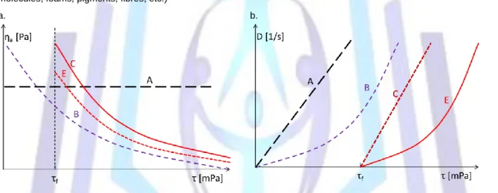
Many fluids behave in a non-Newtonian way in practice. This means their viscosity depends on the shear rate (see Figure 1). The main deviations are caused by the suspension, which contains solid/soft particles (cells, aggregates, large molecules, foams, pigments, fibres, etc.)

a. b.

Figure 1. These flows could happen in various circumstances (ηa = τ/D is the apparent viscosity). (A) Newtonian flow, ideal viscous, D = τ/η; (B) Oswald flow, pseudo-plastic, power law D = k τⁿ (n > 1), (C) Bingham flow, ductile, D = ( τ – τf )/η; (D) Casson flow, ductile, D=( τ^½ – τf½

)²/η. The healthy blood is Bingham fluid (C).

Of course the shear rate versus shear-stress depends on the concentration of the solid/soft particles in the actual suspension (see Figure 2).

Figure 2. Development of the non-Newtonian behavior of the fluid due to the growing concentration of the solid/soft particles

The rheology of blood is non-Newtonian, meaning that the blood has a non-linear shear-stress to shear-rate relationship.

The blood is also a suspension, where the suspended “particles” are cells (predominantly erythrocytes) in electrolyte of various ions. This property is determined by the composition of blood, and by the particular concentration of its components. The behaviour of the flow of blood differs considerably from that of simple suspensions. The main difference is the dependence of the flow on the shear-strength. There are two key reasons for this:

1. At low velocities, the cells aggregate and the liquid has a high viscosity. The aggregates are eroded in the case of a shear rate of D = 10–20/s and the apparent viscosity of the blood drops.

2. The erythrocytes behave like liquid drops at high shear rate (D > 100/s), which decreases the apparent viscosity too.

They key factors determining the actual viscosity of the blood are:

- The viscosity of the blood-plasma, in which the dissolved proteins are mainly globulins and fibrinogens. The albumin has a weak influence on the viscosity of the plasma;

- The volume percentage of haematocrit;

- Deformability of erythrocytes;

- Aggregation ability.

The effect of the last two points is shown in Figure 3., where the viscosities of erythrocytes of healthy blood (A) and blood suspended in salt solution (unable to aggregate) and processed with formaldehyde (unable to be deformed) (B) are compared. It shows clearly that the processed blood is a Newtonian liquid, while the healthy blood is not. It appears that the non-Newtonian property of the blood could be important for healthy functioning.

Figure 3. Effect of aggregation and deformability on the viscosity () versus shear rate (D). (A) healthy blood, (B) blood suspended in salt solution (unable to aggregate) and processed with formaldehyde (unable to be

deformed)

Consequently the healthy blood is certainly a non-Newtonian liquid. The shear stress could be described by a power-law function (Oswald fluid) [1]:

dz D du

KD



 ,



where D is the shear rate, which is related to the gradient of the flow velocity (u). K and n are characteristic constants, depending on the composition of the blood [2]:

 





2 3

1

,

b b

b

a a a

Fibrn Chol

Hct b n

Fibrn Chol

Hct a K





where the abbreviations denote the concentrations of the haematocrit, cholesterol, and fibrinogen. Their values are listed

Table 1. Parameters of healthy and non-healthy blood

Constants Healthy control Cerebrovascular accident

A 0.0022 0.0435

a

a

a

b 2.1750 0.9969

b

b

b

Equation (2) fits the experimental data in the interval of shear rates of 0–100/s with the data in Table 1.

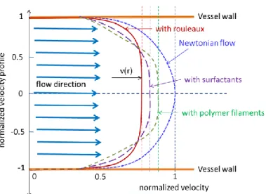
Aggregation of the blood is a well-known phenomenon. This process controls the optimal flow conditions in the environment of the actual vessel. The long-chain fibrinogen or dextran is absorbed on the surface on more cells, leading to aggregation [3] (mostly rouleaux formation [4]). The tendency toward aggregation increases due to the decreasing blood flow in venous vessel networks [5]. In this way, the behaviour of the blood flow tends toward Bingham liquids by increasing the deviation from the classical Newtonian liquids (see Figure 4.) [5].

Figure 4. Velocity profile of the blood flow. (A) The classical laminar flow follows a parabola, while (B) when the blood has aggregates and the velocity is slow, the deformation of the profile becomes more and more flat and

similar to the profile of solids.

The healthy blood is a pseudo-plastic power-law type non-Newtonian liquid. The formation of the profiles develops over time even during constant stress [6].

The so-called cork flow is created in the region where the shear-speed is lower than the threshold. Here the layers of the liquid do not have relative motions. (The Newton’s flow has no such region.) It is clear that the region of the cork flow favours the RP, the large structures could be formed without relative movements, without shear-stress. In the Newton’s flow the RP is instable, its size decreases. The various substances in the blood modify the cork-profile, (see Figure 5.).

The blood rheology has crucial role in RP formation, [7].

Figure 5. Cork-profile of the velocity of blood flow with various intermixtures (RP, surfactants, filaments) The apparent viscosity of the non-Newtonian liquid decreases by the shear-rate, and its apparent viscosity decreases with the shear rate, and in perfect state it is no longer an Oswald fluid but a Bingham fluid. This is a Bingham type liquid described by the following equation [8]:

 

 

 

















 dr

D

dv

f

(3)

where τ is the shear stress and τf is the shear threshold value, because the blood behaves in a non-viscous way at low shear stress. In Table 2, we list some experimental data [9], which fit the curve described by Eq. (4), as shown in Figure 6.

(the accuracy of the fit is > 0.99).

Table 2. Relation between the shear rate and shear stress in the case of healthy blood

  s

D 1 /

 mPa 



 ^mPa  ^{ 17 , 474  4 , 834 D}   ^{1 / s}



Figure 6. Viscosity (η) versus shear rate (D) based on experimental data [9]

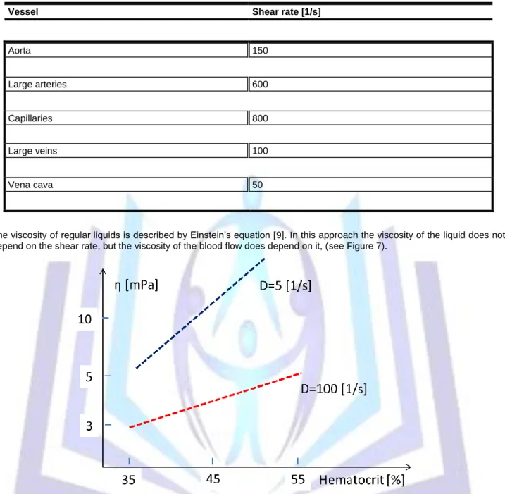
Low viscosity is necessary for optimal energy transport by the blood flow, so a high shear rate (D) is preferred. The various shear rates in different vessels in regular conditions are shown in Table 3.

Table 3. Shear rate in various blood vessels

Vessel Shear rate [1/s]

Aorta 150

Large arteries 600

Capillaries 800

Large veins 100

Vena cava 50

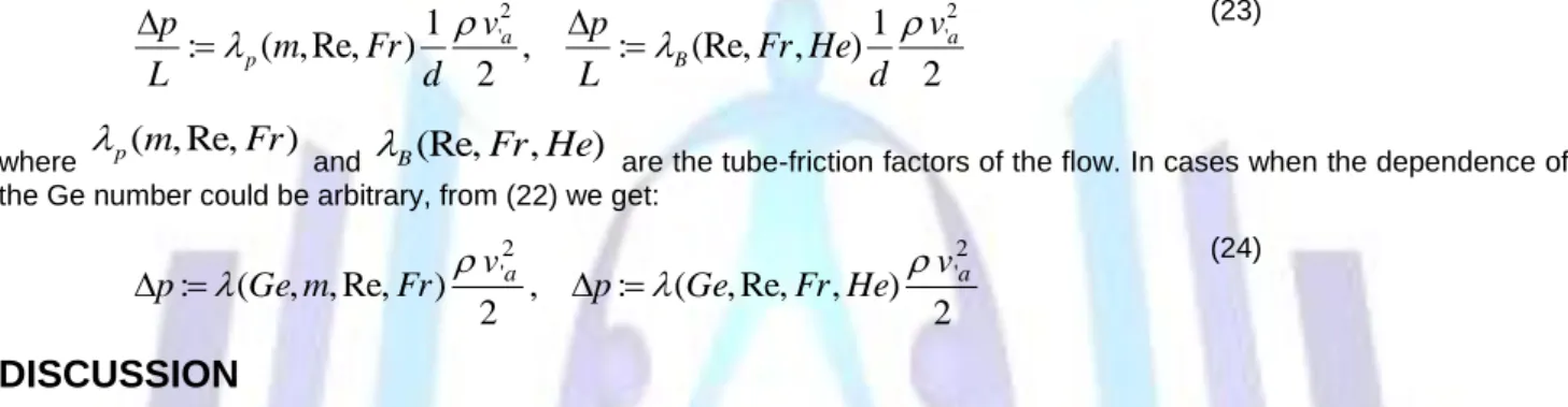
The viscosity of regular liquids is described by Einstein’s equation [9]. In this approach the viscosity of the liquid does not depend on the shear rate, but the viscosity of the blood flow does depend on it, (see Figure 7).

Figure 7. Viscosity of the blood () versus concentration of haemocyte volume percentages at different shear rates (D)

The complex fluid mechanics of non-Newtonian liquids is also very numerically complicated, so its complete solution with numerical analysis is missing as well. The flow characteristics are measured and the experimental investigation is the focus of the research. However the experiments are frequently applied on model systems, which are not identical to the real situations under study, and the similarities are studied. This is why the principles of analogy of the flows in model conditions are applied.

The conditions of similarity in the case of non-Newtonian flows are the geometric and dynamic similarities. The flow and its changes are described by dynamic equations, which are fixed by their initial and boundary conditions. The equivalence of these means Identical equations of material and momentum balances in the similar flows.

METHOD

The various sizes of the vessels can be described well when we know the conditions of similarities of the flows [10]. Let us study the similarities of the flows in Bingham-like healthy blood. We compare the actual task with a smaller sample flow characterized by the parameters shown in Figure 8.

Figure 8. Parameter sets for the study of the similarity The momentum balances of the parameters in Fig. 8 are

dA dA

p dV f dV v

A A

V V















   









and

, , , , , , ,

, ,

, ,

, ,

dA dA

p dV

f dV

v

A A

V V















   









Due to the small sample volumes, we apply the principle of averaging of the integrals:

A A

p V f V

v           

 



and

, , , , , , , ,

,

 v   V  f   V  p   A     A



RESULTS

The values in Eqs. (7) and (8), are averages, but for simplicity (due to the small volume for averaging) we consider their equality with the actual values.

The relationship between the small sample and the actual flow are

, '

, '

, '

, '

, ' , ' , '

f C f C

p C p C

v C v t C t L C L

f

p v

t L

























 (9)

where L and L’ are the characteristic sizes of the diameters of the small sample and the actual system, and the constants CL, Ct, Cv, Cp, Cτ, and Cf denote the ratio of the parameters.

The C constants have some relations, because the length, time, and velocity are not independent:

t L

v

C

C  C

Substitute (9) into the balance equation (8), we get:

V C f

C C C C A

C A C C p

C V C v

v f L v

v

p

           





















where we know from (7) that the criterion equations are

, 1 ,

1 ,

1

2

  

v f v

v p

C C

C C

C C C

C C









(12)

which we considered in order to calculate (11).

The following expressions have to be equal, when the power-law similarities like in (1) are considered::

m

m

K D

KD , '  ' '

 



Introducing the ratio

C

,

K C

K ' 

From Eqs. (9) and (13) we get:

m

L v k

C C C C  

 



 

 (15)

Substituting this into (12), we obtain the criteria equations:

, 1 ,

1 ,

1

2



 

v f m L

L m v

K v

p

C C C C C

C C

C C

C C







(16)

Together with the geometrical similarities, these conditions fix the similarity of the flows.

Reformulating (16) by using (9), well-known constants can be introduced:

' ' ' ' :

' , ' ' : '

Re , ' ' : '

2 2

2 2

L v f L v f Fr

K L v K

L v v

p v

Eu p

m m m

m

























where Eu is the Euler number, Re is the Reynolds number, and Fr is the Froude number. In the case of corresponding similarity numbers, the two flows are similar.

The similarity numbers in Bingham fluids using Eq. (3) describe the equality of the following equations:

' ' ' '

, D

D

f

   



    

Introducing



 '  C

and considering (9), from (18) we get:

1 ,

1 











C C

C C C

C C C

v L v

L ^f

(18)

In this case the conditions shown in (12). the similarities of Bingham fluids need:

2 2 2

2 2 2

' ' ' : '

' , ' ' ' :

' , ' ' : '

Re , ' ' : '





























L He L

L v f L v f L Fr

v vL v

p v

Eu p

f

f

















(20)

where an additional constant, the Hedström number He, appears.

Because the dynamic equation of the flow makes a relation between the physical properties of the fluid flow, the above

constants are not independent. Denoting the geometric similarity number by Ge, in the case of tubes

d Ge :  L

, where L is the length and d is the diameter of the tube, then the following connections can be established and the power (Eup) and Bingham flow (EuB) can be measured experimentally:

) , Re, , ( : ),

Re, , , (

: F Ge m Fr Eu F Ge Fr He

Eu





In practice the Darcy-Weissbach resistance principle applies for tubes, where the functions depend linearly on the length of the tube, and equations (21) will be:

) , (Re, :

), Re, , (

: Fr He

d Eu L Fr m d G

Eu

 L



When the characteristic behaviours that are of interest to us are the pressure difference and average speed difference of the flow between the two ends of the tube actually studied, using Eqs. (17) and (20) we get:

2 ) 1 , (Re, :

2 , ) 1 Re, , ( :

2 ' 2

' a

B a

p

v He d L Fr

p v

Fr d L m

p       



where



( m , Re, Fr )

and



(Re, Fr , He )

) 2 , Re, , ( : 2 ,

) Re, , , ( :

2 ' 2

'a

v

He Fr Ge v p

Fr m Ge

p       



DISCUSSION

When the flow velocity decreases in one of the vessels working in parallel with others in anetwork, the viscosity there will increase and the blood flow could be completely blocked, causing hypoxia and its complications.

When the blood flows in vessels with diameters smaller than 100 m, it is a microcirculation situation. Here the important phenomenon is the dependence of the viscosity on the diameter of the vessel (see Figure 9).

Figure 9. Dependence of the viscosity of the blood on the internal diameter of the vessel

The reason for this effect is that the large shear rate concentrates the erythrocytes into the axis of the vessel due to the Magnus effect, so their concentration decreases in the boundaries and therefore the viscosity decreases too. In thicker vessels this effect does not exist, due to the smaller shear rate, so the viscosity increases at the boundaries in those vessels.

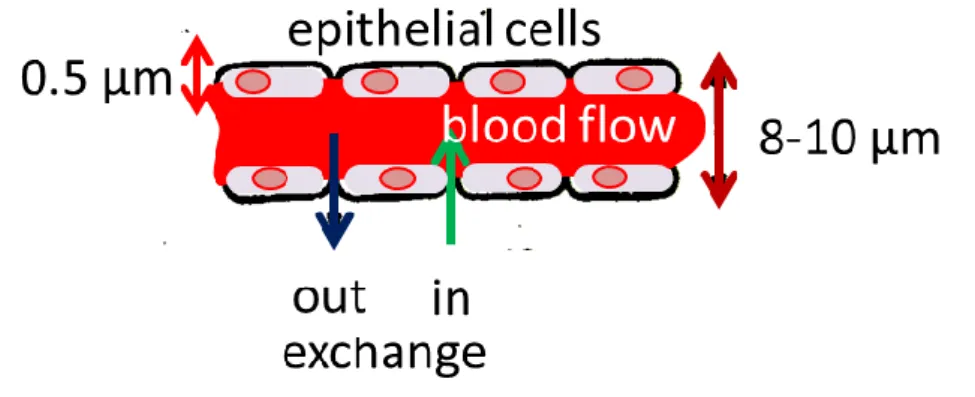
In general, capillaries are 400–700 μm in length and 8–10 μm in internal diameter. Loosely connected endothelial cells form their walls, which are 0.5 μm thick (see Figure 10).

Fiure 10. Construction and material exchange of the capillaries

Capillaries have a two-way exchange of electrolytes with their environment: in- and out- exchanges. The actual direction depends on the flow in the capillary, the osmotic pressure of the capillary, and the actual interstitial fluids. The osmotic pressure is ~2.6 kPa but at the beginning of the vessel it is ~4.0 kPa, so here the out-flow determines the exchange, while at the end of the capillary the pressure is only ~1.3 kPa, leading to the opposite exchange direction. The volumes of the incoming and outgoing fluids are different, and the difference is equalized by the actual lymph flow. The osmotic pressure of the capillary is predominantly created by the proteins (albumin and four globulins) in the blood. When the amount of proteins decreases (e.g. due to the occurrence of inflammation or other irregularities), the outward movement of proteins from the vessel decreases the osmotic pressure of the interstitial fluid, suppressing the movement of fluids into the vessel.

The blood pressure of the flow has a significant influence on the optimal work of the heart. Under regular conditions, the control of the blood pressure predominantly occurs in the aorta, and the muscles of vessels govern the overall cross- sections of the vessels. The flow speed, vessel diameter, and pressure comparison are shown in Figure 11.

Figure 11. Changes of velocity (v), overall cross-section (A), and pressure (p) in the blood-vessel network The blood flow can be described well by the Bingham fluid model shown in (3). The differential momentum balance is:

 0



 dx

dp r dr

d  

Its solution on the shear-stress is:

  dx

dp r r

 2



showing that the shearing is largest at the wall of the vessel:

dx dp R

W

 2



The dynamic equation obtained by substitution of (3) into (25) is:

0 ) 0 ( 2 ,

1  



 v R

dx dp r dr

dv







(28) Its solution is:

 R r   R r 

dx r dp

v   









2 2

4 ) 1 (

(29)

when the following condition is valid:

dx

dp r   2

(30)

From here, the radius where the flow is real is:

R dx

r dp r

F f f





 



 2

0

(31)

In the interval

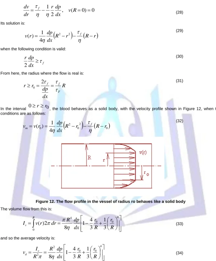
0  r  r

, the blood behaves as a solid body, with the velocity profile shown in Figure 12, when the conditions are as follows:

  



2 0 2

0

4

) 1

( R r R r

dx r dp

v

v

   









(32)

Figure 12. The flow profile in the vessel of radius ro behaves like a solid body The volume flow from this is:

 





 



 



 



 





 

0

3

1 3 1 4 2 8

)

( R

r R r dx

dp dr R

r v I

R

v



 

and so the average velocity is:

 





 



 



 



 







4 0 0

2

2

3

1 3 1 4

8 R

r R r dx

dp R R

v

I





We suppose that the blood has a laminar flow, fixing the direction of the velocity and the shear stress. However, in some cases (e.g. stenosis, or strong vasocontraction) the velocity of blood increases remarkably and the viscosity of the blood decreases, forming turbulent flow. The well calculable laminar situation changes and the deterministic flow is transformed to a chaotic one. In this case the physical parameters are not fixed values, but probabilities, stochastic variables and only the probability parameters can be determined (e.g. mean, deviation).

The turbulent flow of non-Newtonian fluids is less clear due to experimental complications. One of the important results of turbulent blood flow is that the critical Reynolds number (Recrit) depends on the flow exponent, according to Table 4 [1].

Table 4. The critical Reynolds number versus flow exponent

n 1 0.38 0.2

Recrit 2100 3100 5000

Importantly, the critical Reynolds number for a Newtonian fluid like water (n = 1) is smaller than that of blood, so water beings to exhibit turbulence earlier than blood does.

The formation of a boundary layer is a characteristic phenomenon in both Newtonian and non-Newtonian flows (Prandtl’s boundary principles). This makes it possible to divide the flow volume into two domains with the relative movement of the solid wall and the fluid. The friction in the domain near to the wall has a remarkable role, while the domain inside the tube has negligible friction and the flow behaves ideally. In the wall-domain the viscous stresses have a significant role, irrespective of whether the fluid is Newtonian or not; while in the internal domain they are negligible due to the small values of the shear rate. The conditions of the flat wall are shown in Figure 13.

Figure 13. Formation of boundary conditions. For simplicity we model it by a flat wall. The model shows the development of the turbulent flow from left to right. Until the edge of a position xcrit the flow is laminar.

From here the flow transforms gradually to turbulent, and the ordered flow starts to become disordered in the majority of the volume of the flow. Only a gradually thinner layer exists where the flow remains laminar

(laminar boundary layer).

The flow from the point when it enters could be stable, (remains laminar); or form turbulent phases (see Figure 14).

Figure 14. Stabilization of stationary flow in vessels

Over a thin laminar boundary layer, where the viscous stresses have a role, the flow transforms to turbulent. Various transition intervals appear between the two dynamic situations. The actual locations of the transition are determined by the environmental conditions or the connected flows. The average time of the velocity changes is only very small, so the viscous stress is negligible here. The turbulent stresses (originating from the time fluctuation of the velocity) play the main governing role in the turbulent region. The order of magnitude of the two stresses in the boundaries is approximately equal.

The friction on the vessel wall of blood during laminar flow is:

2

: 1

v

D L

p dx

p d

 

 



(35)

So the vessel-friction parameter is:

4 2 3

2

3 Re

64 Re 6 1 64 Re

1 



 



 



 He He





from which Re and He can be determined. The turbulent flow of the blood can be approximated well by:

5

b

, Re 10

Re

a 





where

15 , 0 l 48

, 0

l

, b 0 , 25

316 , 0

a 



 







 

 

 







 

(38)

Note that the apparent and dynamic viscosities are equal in the case of Newtonian fluids, so (38) satisfies the Blasius equation:

4 1

Re 316 ,

0





CONCLUSION

Using the classical field approach, the blood flow is described in detail. The basic balance equations and general non- Newtonian criteria of the blood flow are established, together with the flow similarities, in order to study the blood flow in vessels of various sizes.

REFERENCES

[1] Krell, Ug. S., Schirser, W. 1987. Nicht-Newtonsche Flüssigkeiten, VEB Deutscher Verlag für Grundstaffindustrie.

Leipzig.

[2] Hussain, M. A., Puniyani, R. R. 1999. Relationship between power law coefficients and major blood constituents affecting the whole blood viscosity. J. Biosci. 24(3), 329-337.

[3] Chien, J. 1973. Ultrastructural basis of the mechanism of rouleaux formation. Microvasc. Res. 155-166.

[4] Faitelson, L. A., Jakobsons, E. E. 2003. Aggregation of erythrocytes into columnar structures ("rouleaux") and the rheology of blood. J. Eng. Phys. Thermophysics. 76(3):728-729.

[5] Bishop, J. J. 2001. Rheology effects of red blood cell aggregation int he venous network: A review of recent studies.

Biorheology. 38:263-274.

[6] Böhme, G. (1981) Strömungsmechanik nicht-newtonsche Fluide. Teubner-Verlag, Stuttgart.

[7] Faitelson, A., Jakobsons, E. E. 2003. Aggregation of erythrocytes into columnar structure (“rouleaux”) and the rheology of blood. J. Eng. Phys. Thermophysics 76:728-742.

[8] Harper, J. C. 1976. ASAE Paper No. 66-837. Am. Soc. Agr. Engrs. Saint Joseph, Michigen.

[9] Astarita, G., Marucci, G. 1984. Principle of Non- Newtonian Fluid Mechanics. McGraw-Hill, New York.

[10] Becker, H. A. 1976. Dimensionless Parameters. Applied Science Publishers, London.

Author’ biography with Photo

PD Dr. Oliver SZASZ, PhD

Dr. Oliver Szasz is bioengineer, associate professor of Biotechnics Department of St. Istvan University (Hungary). He has over 40 published articles, he owns several patents. He has essential contribution of inventing of nanothermia technology.