C H A P T E R 3
THE RELAXATION THEORY O F TRANSPORT PHENOMENA Taikyue Ree and Henry Eyring
I. I n t r o d u c t i o n 83 I I . Generalized T h e o r y of V i s c o s i t y 88
1. H e t e r o g e n e i t y of F l o w Units 88 2. I n c o m p l e t e E q u i l i b r a t i o n of the A c t i v a t e d C o m p l e x 89
3. T h e E q u a t i o n of State for F l o w Units Using the Virial T h e o r e m 90
4. Generalized V i s c o s i t y F o r m u l a 91 5. D e f o r m a b l e F l o w Units 92
a. E n t a n g l e m e n t - D i s e n t a n g l e m e n t Transition 92
b. a-ß Transition 94 c. P r i m a r y C r e e p 96 I I I . A Generalized T h e o r y of Diffusion 97
1. T h e R e l a t i o n between V i s c o s i t y and Diffusion 97
2. Free Diffusion 99 3. Stokes-Einstein E q u a t i o n 100
4. M e m b r a n e Diffusion 101
I V . A p p l i c a t i o n s 105 1. Solid Plastic S y s t e m 105
a. D e t e r m i n a t i o n of the Parameters 106
6. Results 107 c. Discussions I l l 2. Solution S y s t e m of H i g h P o l y m e r s 114
a. V i s c o s i t y Formulas for Solution Systems 114
b. Results 115 c. Discussions 128 3. D e f o r m a b l e Systems 131
a. Classification of F l o w Curves 131
b. Ostwald C u r v e 132
4. M e t a l s 134 5. Diffusion in Solution 136
V . N a t u r e of " H o l e s " 138 1. Structure of L i q u i d s 138 2. M e l t i n g of Solids 141 3. T h e V o l u m e P r o v i d i n g an A d d i t i o n a l E q u i l i b r i u m Site 142
N o m e n c l a t u r e 142 I. Introduction
W e treat in this chapter the transport p h e n o m e n a in condensed systems from the v i e w p o i n t of rate processes. T h e molecules ( a t o m s , ions, m o l e c u - lar segments) in a condensed phase o c c u p y positions of equilibrium, and
83
8 4 T A I K Y U E R E E A N D H E N R Y EYRING
may be considered as vibrating about the minimum of a free energy well.
T h e structure of all condensed systems may be thought of as possessing a more or less regular lattice arrangement. T h e regularity of the lattice is different from substance to substance. There are many substances which have well-defined regular lattice structures; solid crystals belong to this category. On the other hand, the lattices of liquids are less regular, i.e., there are many empty equilibrium places in the lattices; such lattices are readily deformable. Even in solid crystals, however, the lattices are in- complete because of dislocations and crystal imperfections.
T h e effect of a stress on a b o d y is to cause displacements from equilibrium along the various planes separating molecular layers. If the b o d y is per- fectly elastic, the stored potential energy is immediately and completely re- leased when the stress is released. T h e result is the immediate and complete return of the molecular patches to their original minimum positions in the energy wells. Thus, the elasticity modulus, shear modulus, bulk modulus, and hardness are all functions of the steepness of the energy wells. H o o k e ' s law describes the relation between the stress and the displacement in this case when these quantities are relatively small.
If a relatively large stress acts constantly on a b o d y , however, molecular patches on the t w o sides of a shear plane j u m p with respect to each other over the energy barrier, and take up the neighboring new equilibrium posi- tion. In this way the energy stored up in stress is released as thermal energy.
This statistical displacement of patches b y jumping along shear planes con- tinues as long as the stress acts, i.e., the substance flows in a direction to release the stress. In this way permanent deformation occurs. This relative displacement to new equilibrium positions along shear planes we call the relaxation theory of transport phenomena. A s we shall see later, diffusion is to be thought of as a multiple shear process.
Before presenting the recent achievement of the relaxation theory in this field, it would be advisable to depict the fundamental results reported in papers, reviews and monographs. Consider that shear occurs along sets of parallel shear layers. T h e distance between these layers is represented b y the symbol λ ι . T h e stress (shear force per unit area) is indicated b y / . Let λ be the distance of two equilibrium positions for patches in the direc- tion of shear, the distance between neighboring patches in the same direc- tion being λ2 ; the latter is not necessarily equal t o λ. Finally, the mean dis- tance between two adjacent flowing patches in the moving layer in a direction at right angles to the shear is λ3. Eyring1, la represented the shear
1 H . Eyring, J. Chem. Phys. 4, 283 (1936).
l aS . Glasstone, Κ . J. Laidler, and H . Eyring, " T h e T h e o r y of Rate Processes,"
pp. 477-551. McGraw-Hill, N e w Y o r k , 1941.
R E L A X A T I O N T H E O R Y O F T R A N S P O R T P H E N O M E N A 8 5
rate s in this ease b y
where a symmetrical potential barrier was assumed for the flow process.
I n equation ( l a ) k' is a rate constant for the jumping patches when n o stress is acting, that is
k
f=
κ —jjr- exp ( - Δ ί7* ) (16)h
where AFt is the activation free energy for the flow process. According t o the definition of viscosity, 77, the latter is given as the ratio of stress t o strain rate. Thus, from equation ( l a ) , we obtain
β sinh"1 ßa
V = ττ.
OL ßs where,
( 2 )
a = 2kT ( 3)
and
T h e properties of the function s i n h- 1 (ßs)/(ßs) are as follows:
r s i n h- 1 ßs 1 / rN
lim
— =
1 ( 5 ) /3s->0 ßSlira
s i n tf = 0 ( 6 )
ßs-too ßS
T h u s , at l o w stress and l o w shear rate, viscosity is given according t o equa- tions ( 2 ) and ( 5 ) b y
while at high values of / and s, the viscosity approaches zero. T h e viscosity expressed b y equation ( 7 ) is called N e w t o n i a n viscosity, i.e., the viscosity is independent of stress and shear rate. N o n - N e w t o n i a n viscosity is ex- pressed b y equation ( 2 ) , i.e., the v i s c o s i t y decreases with stress and shear rate.
86 T A I K Y U E R E E A N D H E N R Y E Y R I N G
W e represent Newtonian viscosity b y η8, the subscript s indicating the conditions of small values of stress and shear rate. Introducing the expres- sion for ¥ into β, one obtains from equation (7) the following formula:
_ hN làrhlRT / Q N
Vs y e {#)
Here the approximations λ ~ λι ~ λ2 o^. λ3 and λ3 ~ V/N were made, where V and Ν are the volume of one mole of flow patches and the A v o - gadro number, respectively. Powell, Rosevear, and Eyring2 found the rela- tion
AEV&V/AFX = 2.45 (9)
where AEVSLP is the vaporization heat of a liquid. Equation (9) holds for nearly 100 substances, excluding metals but including associated liquids.
Thus, the Newtonian viscosities of many liquids at atmospheric pressures are calculated with good results, using the values of V and AEy&v . Plotting the activation heat for viscous flows 2?Vi e, against vaporization heats, the same authors2 found the relation
E v is = (10)
η
where η ~ 3 for nonassociated liquids, while η ~ 4 for associated liquids.
For metals, the value of η changes from 8 t o 25 or more. This is due t o the fact that the unit in the vaporization of metals is the neutral atom, while the unit for viscous flow is the much smaller metal i o n .l b'2
W e must still discuss the effect of pressure on viscosity. Generally, vis- cosity increases with the pressure at constant temperature. This fact indi- cates that activation free energy for flow processes increases with the pres- sure, p. F r o m well-known basic considerations the dependence is given b y the following equation:
AF* = AF1X + Γ dp ~ AFj + pAVt (11) Jp=l
where, AV* is the mean volume increase accompanying the activation, and AFi* is the activation free energy at ρ = 1. Using the viscosity data at high pressures obtained b y Bridgman3 Ewell and Eyring,4 and Frish et al.b determined the activation free energy, AFl. Plotting AFl against p, these authors determined AVX from the slope of the straight line of the
2R . E . Powell, E . Rosevear, and H . Eyring, Ind. Eng. Chem. 33, 430 (1941).
3 P. W. Bridgman, " T h e Physics of High Pressures." Macmillan, N e w Y o r k , 1931.
4 R . H . Ewell and H . Eyring, J. Chem. Phys. 5, 726 (1937).
5 D . Frish, H . Eyring, and J. F. Kincaid, Appl. Phys. 11, 75 (1940).
R E L A X A T I O N T H E O R Y OF T R A N S P O R T P H E N O M E N A 87 diagram [cf. equation (11)]. T h e y found the following relation:
(12) where nf ~ 7 for nonassociated liquids, and n' 21 for liquid metals.
T h e physical significance of these results is interesting. A s previously mentioned, the relaxation theory assumes the presence of empty sites, or
"holes," in condensed systems. If there are no holes available, flow does not occur. T h e energy needed for the formation of the hole is a function of the bond strength between molecules. The activation heat for viscous flow is used mostly for the formation of the new hole. T h e change of volume, Δ 7*, in equation (11) is associated with the formation of the new hole.
According to equation (12), the size of the new hole is considered as Y normal molecular volume for nonassociated liquids, while as the normal volume for metals. T h e very small hole volume for metals is probably due to the fact that in metals the flow units are ions which are 3^3 the normal neutral atoms in size.
T h e energy required t o make a hole of molecular size in a liquid is equal to the vaporization heat, Δ £ 7ν αρ ,1 If we assume that (1) the energy re- quired to make the new hole which is needed for viscous flow is propor- tional to the size of the hole, and that (2) all of the activation energy is spent to make the new hole, then equation (10) would indicate that the size of the new hole is about Y% the normal molecular volume for nonasso- ciated liquids. This result must be reconciled with the value found from equation (12), i.e., the size of the new hole is % the normal molecular vol- ume. This seeming contradiction arises from our first assumption, which is not true. Rather one must assume that the energy required to make the hole of size V/7 is AEvap/3, instead of AEvap/7. Actually, these holes, a fraction of molecular size, are more expensive per unit volume because neighbors presumably bond more poorly with each other than in a perfect lattice as a result of poorer fit as well as because of the absence of bonding to a lacuna.
Walter and Eyring6 calculated the potential energy of a condensed sys- tem, Εy as a function of the numbers of moles of holes, f, per mole of mole- cules. W h e n f is very small, the result was
Ε = Es(l - f ) (13) while it turns out to be
(14)
6 J. Walter and H . Eyring, J. Chem. Phys. 9, 393 (1941).
8 8 T A I K Y U E R E E A N D H E N R Y E Y R I N G
under the condition that 2f » \/(n' — 1 ) , which is nearly true in the nor- mal liquid range. In equations ( 1 3 ) and ( 1 4 ) Es is the potential energy per mole of the solid of the condensed system (the gaseous phase being taken as reference), ν and vs are the volumes per molecule in the liquid and solid, respectively, n' is a constant which is numerically equal t o 8 . 3 5 . Thus, ac- cording to equation ( 1 3 ) , the first holes to be introduced into a solid cost the amount of energy required to vaporize a molecule from the solid. T h e volume difference, ν — vs, is considered proportional t o the number of holes in the liquid. Thus, equation ( 1 4 ) shows that the energy of vaporization of a liquid does not decrease linearly with the number of holes. Consequently, it is wrong t o assume that the energy required to make a hole is propor- tional to the size of the hole.
T h e nature of the holes is very important in the relaxation theory of transport phenomena. W e will return to this problem later.
T h e fundamental equations in the relaxation theory, ( l a ) , (lb), ( 2 ) , and ( 8 ) , were derived under the following assumptions: Firstly, the flow system is homogeneous, being composed of only one kind of flow unit. Secondly, the activated complex for flow is in complete equilibration with ambient temperature. This situation, however, is rather a special one, there being many cases where the system has heterogeneous flow units. W e must, there- fore, generalize the old theory of relaxation.
1. H E T E R O G E N E I T Y OF F L O W U N I T S
Consider, for example, a shear plane in a sheet of rubber. T h e flow patches may consist of segments of a molecule, whole molecules, or several mole- cules shifting as a unit. One m a y see then that there are many kinds of flow units which differ in the degree of entanglement, which a flow patch has with the patches on the opposite side of the shear plane. Some flow units will not have any bonds except van der Waals' bonds acting across the shear plane, while others have such bonds. T h e t w o kinds of flow units will be referred t o as nonentangled and entangled units, respectively. Heavily entangled units will resist the shear more strongly than lightly entangled ones. T h e relaxation time of a flow unit is defined as the reciprocal of the rate constant for the flow of the unit, i.e., 1/fc'. T h e heavily entangled units have large relaxation times while the converse is true for the lightly en- tangled units. All flow patches involve the quantity β = ( ^ ) Α Λ which is the relaxation time multiplied b y a dimensionless factor. Since this unknown factor is probably near unity, it will be convenient to speak of β itself as the relaxation time.
II. G e n e r a l i z e d Theory o f Viscosity
R E L A X A T I O N T H E O R Y OF TRANSPORT PHENOMENA 8 9
ο
Rote of shear (s)
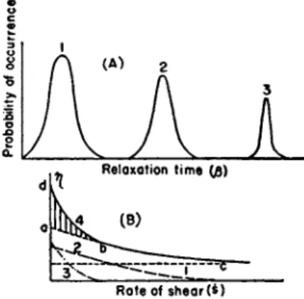
FIG. 1 A . Probability of the occurrence of flow units vs. relaxation time.
FIG. I B . Viscosity vs. shear rate. Actual viscosity is composed of the contribution from three groups of flow units. Curve 1: 7 7 = χφ\/α\ . Curve 2 : η = {x$2/a2) s i n h-1
0 2 s / ( 0 2 s ) . Curve 3 : ^ = {x^ßz/az) s i n h- 1 /83s/(j83s). C u r v e 4 : Superposition of Curves 1, 2 , and 3 .
W e consider that a flow system is c o m p o s e d of several groups of flow units. E a c h group is characterized b y an average relaxation time, ßn . W e frequently find marked variations such as βι <<C ft <5C ßz. E a c h ßn is an average for a closely related set of relaxations. T h e relaxation time spectrum is as shown in Fig. 1 A , where a near-Gaussian-type distribution p r o b a b l y exists in each g r o u p . W e assume that through the whole range of s in an actual experiment, the following conditions are satisfied:
ßie « 1 ( 1 5 )
ß2e > 1 ( 1 6 )
ß*s » 1 ( 1 7 )
ßns > > > 1 ( 1 8 )
(for n > 4 )
2. I N C O M P L E T E E Q U I L I B R A T I O N O F T H E A C T I V A T E D C O M P L E X
The activated complex, lying at the t o p of the potential barrier, involves m a n y degrees of freedom. These degrees of freedom are in equilibrium with a large number of neighboring oscillators. If the latter behave classically, the mean available energy is kT for each. H o w e v e r , various kinds of in- complete equilibration of activated complex degrees of freedom with ambient temperature are observed in plastic flow. F o r example, in the annealing of a l u m p of glass, the inside flow units are in equilibrium with the local temperature. T h u s , the rate constant for flow is given b y7
7 H . E y r i n g and T . R e e , Proc. Natl Acad. Sei. U. S. 41, 118 (1955).
90 T A I K Y U E R E E A N D H E N R Y E Y R I N G
k' = κ £ exp - Σ (AF^/Ji (19) Here, 7 0 is the mean available energy of those oscillators equilibrating with the translational degree of freedom corresponding to crossing the p o - tential barrier, and 7,· is the same mean available energy of those oscillators equilibrating with the ith group of activated complex degrees of freedom requiring the activation free energy, AF*. If there are classical degrees of freedom equilibrating with all the degrees of freedom of the activated complex, each 7 can be replaced b y kT. In this case, equation (19) reduces to the familiar equation (lb).
As far as the available evidence indicates, it is usually satisfactory to write 7 0 = kT. However, to the approximation that 70 can be identified with the average energy of an oscillator, we have
A t low temperatures this has the value v/2, and at high temperatures the usual value kT/h. T h e essentially frictionless flow of H e l l seems at least in qualitative accord with the low temperature form of equation (21), since there is no evidence that the process ceases at absolute zero in the way indicated b y kT/h. Because of quantum effects at low temperatures, the transmission coefficient, κ, including barrier leakage will be important, and Kjo/h will be best treated as a unit.
3 . T H E E Q U A T I O N OF S T A T E F O R F L O W U N I T S U S I N G T H E V I R I A L T H E O R E M7
Flow units vibrate about their equilibrium positions. The equation of state for the flow units may be obtained b y applying the virial theorem
where X , x, and χ are the force, displacement, and velocity of the flow unit in the x-direction (the direction of relative displacement), m is the mass of the unit, and the bars represent the average over a very long time. Let fo be the local microstress on the flow unit resulting from its surroundings.
T h e microstress is to be distinguished from the over-all macrostress / . Then, the following identifications can be made:
(20)
(21)
Xx = — nix- (22)
X — \2^3fo (23)
and
χ = g\ (24)
R E L A X A T I O N T H E O R Y OF T R A N S P O R T P H E N O M E N A 91 where g is the ratio of the length of free vibration, x, of the flow unit whose area is λ2λ3 t o the distance jumped, λ. Thus, 1/g should approximate the ratio of sound velocity in the solid to that in the gas—a value in the neigh- borhood of 7. Further,
mx2 = ys (25)
From equations (22) t o (25), we obtain
λλ2λ3/οο = ys (26)
This is the equation of state of the flow unit.
4. G E N E R A L I Z E D V I S C O S I T Y F O R M U L A
T h e generalized equation of the rate of shear is obtained b y the substi- tutions of equations (19) and (26) into ( l a ) , the results being
è = -ß sinh af (27)
where
* m h m < 2 S)
\ Λ Ι h / \ ys i=i 7< /
and
ΛΛ2Λ3
a =
-2y7
(30)Here, the quantities with the subscript s indicate the corresponding quan- tities in the shear coordinate.
W h e n there are several groups of flow units, each characterized b y dif- ferent relaxation times, β, the total shear stress / is given as follows
/ = Σ Xnfn (31) n = l
Here, xn is the fractional area on a shear surface occupied b y the nth group of units and fn is the force per unit area acting on the nth group. T h e shear rates of all kinds of units are equal, otherwise the slowly moving units would be left behind. In the latter circumstance, a structural change occurs in the flowing substance. Such changes are not generally observed.
Thus, all the different groups of units are obliged t o m o v e with the same shear rate, s, with differing appropriate stresses on each group. T h e longer the natural relaxation time β, the higher the stress, and vice versa. F r o m
92 T A I K Y U E R E E A N D H E N R Y E Y R I N G
equation ( 2 7 ) , the relation between the stress fn and the relaxation time ßn for the nth group is given b y the formula
fn = I sinh 1 (ßj) (32)
OLn
T h e substitution of equation (32) into (31) yields
/ = Σ - sinh"1 (ßj) (33)
n=l OLn
Dividing both sides of equation (33) b y s, one obtains the viscosity formula
=
Ξϋ^ΐ
si*1*1"1(ftnâ) (
3 4^
n=l O^n ßnS
Equation (34) is the generalized viscosity formula derived b y R e e and Eyring,8 and it has been applied t o a wide variety of cases with g o o d re- sults. T h e properties of the function, s i n h- 1 (ßs)/(ße), have been men- tioned before [cf., equations (5) and ( 6 ) ] . Because of these properties, equation (34) gives Newtonian viscosity when s is very small, while it gives non-Newtonian viscosity when s is very large.
5. D E F O R M A B L E F L O W U N I T S
T h u s far w e have assumed that the structure of flow systems is not a function of time and stress. T h a t is, the structure is the same at any time under any stress. It is, however, a c o m m o n experience for cases t o arise where structural change occurs with time and with stress. T h e fracture of a system b y a force is an example of structure change. W e omit treatment of such time-dependent changes here, but w e consider steady-state stress- dependent flow phenomena. Such systems show thixotropy, birefringence, etc. Here w e extend our generalized flow-rate equation (33) t o systems undergoing structural change.
a. Entanglement-Disentanglement Transition
W e have mentioned that intermolecular entanglement determines the relaxation times of flow units. T h e state of entanglement will not be changed b y low stresses. High stresses, on the contrary, tend t o break bonds which m a y not immediately form again.
W e consider the case where entangled and disentangled units are in kinetic equilibrium, and the system shifts toward disentanglement with increasing stress. T h e free-energy curve for the transition is represented b y Fig. 2, where Ε and D indicate the entangled and disentangled units, re- spectively. T h e transition, Ε —•> Ζ), is promoted b y the elastic energy stored up on the flow unit. Such a flow unit is formally represented as a Maxwell
8 T . R e e and H . Eyring, J. Appl. Phys. 26, 793, 800 (1955).
R E L A X A T I O N T H E O R Y O F TRANSPORT PHENOMENA 93 unit—a spring in series with a dashpot. T h e elastic energy, w, stored up during the relaxation time, r, is given b y
w
-C
fds=q¥-
=cè2 (35)Here, G is the spring constant of the unit, and the relations, / = Gs , and SI = re , were used. Here Si is the strain at the time of relaxation.
Let Ce and Cd be the mole fractions of the entangled and disentangled units at time t, respectively. T h e n the net rate of transition, Ε —» D , is given b y
- ^ = Cek,feliCh2,kT - Cdk'be-(1-ß)ca2lkT (36) at
For an unsymmetrical barrier μ will differ from one-half. k'f and fc'& are the rate constants for the forward and backward reactions at zero stress, respectively. T h e condition of steady flow is that the left side of equation (36) is zero. Thus, w e obtain
_ 1
Ge — j _|_ jç-çCèZ/kT (37)
and
KecèVkT
C d = 1 + Ke^T ) ( 3 8
where the following relations were introduced:
Κ = k'f/k'b (39)
-ACe = ACd or Ce + Cd = 1 (40) In equation (39) Κ is the equilibrium constant at zero stress, and the
quantities AC in (40) are the changes of the concentrations of the en- tangled and disentangled units. T h e substitutions of equations (37) and
R E A C T I O N COORDINATE
FIG. 2 . Free energy curve for entanglement-disentanglement transition.
94 T A I K Y U E R E E A N D H E N R Y E Y R I N G (38) into (33) yield
1 + Kecè2'kT
(41) + Σ - sinh-1 (ßns) Here, the disentangled units are treated as N e w t o n i a n units, and the rela- tion
is introduced, where a is the area occupied b y one unit. If one substitutes the condition, c = 0 [i.e., G = 0 from equation (35)], into equation ( 4 1 ) , the latter reduces t o ( 3 3 ) . T h u s , equation (41) is more general than ( 3 3 ) . I n the a b o v e , w e considered the case where the equilibrium between en- tangled and disentangled units shift t o the side of the disentangled units.
T h u s , the viscosity decreases more rapidly with increasing stress than in the ordinary case. A s will be shown later, w e meet this case frequently in polymeric solutions. A n y thixotropic substance exemplifies this case. On the other hand, there is the opposite case where the equilibrium shifts t o the side of entangled units with increasing stress increasing viscosity. Sys- tems showing this effect are said t o show dilatancy. E q u a t i o n (41) thus covers b o t h the thixotropic and dilatant cases.
b. a-ß Transition
In some cases a phase transition is brought a b o u t b y a stress. T h e a-ß transition in keratin fibers is a famous example. Keratin fibers consist of polymeric chains cross-linked b y disulfide b o n d s . T h e s e p o l y m e r i c chains are polypeptides produced b y the condensation of a- a m i n o c a r b o x y l i c acids. A c c o r d i n g t o A s t b u r y and Street9 and A s t b u r y and W o o d s ,1 0 natural and stretched w o o l present different X - r a y diffraction patterns. T h e crystal- line structure of natural w o o l (hair) is called α-keratin, while the stretched form is called ß-keratin. X - r a y patterns show also that there is a large amount of unoriented material. T h e presence of amorphous regions in w o o l is shown b y the infrared studies of E l l i o t t11 and b y the studies of Steel12 on the change in the tensile properties of w o o l with changing concentrations of L i B r . T h e exact structure of the a and β crystalline forms is still not agreed upon. However, there is near agreement on the 1.5 A . distance per amino acid along the helical axis in α-keratin, and the 3.3 A . distance per amino acid in ß-keratin. T w o types of b o n d s , the h y d r o g e n b o n d and di-
9 W . T . A s t b u r y and A . Street, Phil. Trans. Roy. Soc. A230, 75 (1932).
1 0 W . T . A s t b u r y and H . J. W o o d s , Phil. Trans. Roy. Soc. A232, 333 (1934).
11 A . E l l i o t t , Textile Research J. 22, 783 (1952).
1 2 R . Steel, J. Soc. Cosmetic Chem. 3, 99 (1952).
= (Ca) η (42)
RELAXATION THEORY O F TRANSPORT PHENOMENA 95
'////////////
er ο ω ω tu (Τ
OC
REACTION COORDINATE
(A)
FIG. 3 A . Free energy curve for α-β transition.
FIG. SB. Mechanical model for a flow unit suffering α -β transition.
sulfide cross-link, play important roles in the structure of keratin fibers.
Pauling and C o r e y13 showed that hydrogen bonds are responsible for the formation of the helix in the simple a-keratins.
Burte and H a l s e y ,1 4a Burte et al.uh and Speakman and Peters15 intro- duced the idea of the α-β transition to explain the mechanical properties of keratin fibers. In a recent paper, Ruoff and E y r i n g16 considered this idea in explaining their experimental results for hair in water, formic acid, and dimethyl formamide
[N(CH
3)2CHO].
T h e free energy curve for the α-β transition is shown in Fig. 3A. T h e conditions of the first set of the ex- periments carried out b y Ruoff and Eyring were that the fibers were stretched in water at 15 to 35° C . at a uniform rate to an extension of 3 0 % , in about 5 minutes. In these conditions, the plastic flow was so slow that it could be neglected compared to the aperiodic elongation resulting from the α-β transition. Thus, the flow unit was represented b y a spring in series with an aperiodic element as shown in Fig. SB, the latter being responsible for the α-β transition. T h e rate of the α-β transition under stress / is given b ywhere Ca and Cß are the concentrations of the a and β forms, respectively, ( λ λ2λ3)α indicates the flow-unit parameters belonging t o the aperiodic unit, and μ has the same significance as in equation (36). T h e total strain, s, is the sum of the aperiodic strain, sf, and the spring strain, s". Since the aperiodic strain depends on the number of the transformed ß-forms, the
1 3 L . Pauling and R . B . C o r e y , Proc. Roy. Soc. (London) B141, 21 (1953).
1 4a H . Burte and G . Halsey, Textile Research J. 17, 465 (1947).
1 4b H . Burte, G . Halsey, and J. H . Dillon, Textile Research J. 18, 449 (1948).
1 5 L . Peters and J. B . Speakman, Textile Research J. 18, 511 (1948).
1 6 A . L . Ruoff and H . E y r i n g , Proceedings of International W o o l Conference, Volume D , p . 9, Australia (1955).
dCg
dt
= α *ν
( λ λ 2 λ 3 ) α / /*
Γ Cßk bë/ -(1-μ)(λλ
2λ
3)
α//*Γ
(43)96 T A I K Y U E R E E A N D H E N R Y E Y R I N G
following relations hold:
C9 = 4- (44)
C a = 7 s
'
(45)ρ = s + è" (46)
where ρ is the strain rate of the fiber which was kept constant in these ex- periments, and s'oo is the strain where the a —» β transition is completed.
Substituting equations (44) to (46) into (43), one obtains
ρ _ è" = (8; _ s')Kk'^f - s'k'be-2(1-»)a'af (47) where Κ = k/f/k/b and aa = ( λ λ2λ3) α/ 2 ^ Τ . According to H o o k e d law, the
equation
/ = 0(8)8" (48) holds for the spring, where for the general case the spring constant, (7, was
considered to change with strain. From equation (48), one obtains
' • - h i «
T h e substitution of equation (49) into (47) yields the result
ρ ( ι _ i . dJ>i = (S'M _ s')KkV^f - s W -l ) a°f ( 5 0 ) which is the general differential equation for extension of wool fibers at a rapid rate. Using equation (50) Ruoff and Eyring analyzed their experi- mental curves, and showed that under the experimental conditions pre- viously mentioned the a —> β transition is the principal factor for flow in the elongation of keratin fibers.16'17
c. Primary Creep
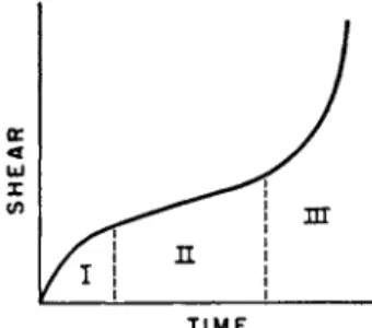
T h e creep curves of solid materials under a constant stress follow usually the form shown in Fig. 4. T h e curve is composed of three parts—I, II, and I I I . In part I, the strain rate, s, decreases with time; in II, s is about con- stant; and in III, s increases rapidly with time, and eventually breakage occurs. T h e parts I, II, and I I I are called the primary, secondary, and tertiary creep, respectively.
It is considered that during primary creep a structural change is brought about b y the stress. B y this change, the material becomes more resistant to flow, or work-hardens. Work-hardening is very important in engineering;
1 7 A . L. Ruoff, dissertation, University of Utah, Department of Chemistry (1955).
R E L A X A T I O N T H E O R Y O F T R A N S P O R T PHENOMENA 9 7
T I M E
FIG. 4 . Creep curve under a constant load; shear vs. time.
however, it is still not fully understood, and will not be treated further here.
T h e secondary creep occurs during steady flow, while primary and tertiary creeps are transient phenomena.
III. A G e n e r a l i z e d Theory of Diffusion
1. T H E R E L A T I O N B E T W E E N V I S C O S I T Y A N D D I F F U S I O N
Diffusion results from a suitable succession of shear displacement pro- moted b y free-energy (chemical potential) gradient. W e assume that at the initial position the diffusing molecules have a concentration, C, an activity coefficient, 7 , and a rate constant of jumping forward to the next equilibrium position, ¥j , which is given b y1'2
k'f = k' ~ = k' —Ί—- (51α)
7 + ay λ
Ύ +ά 2
- 4 - " - ΐ - 7 ) ) ( 5 i t
Here, k' is the rate constant in an ideal system, 7 * is the activity coefficient of the activated complex lying half-way between t w o equilibrium posi- tions; the distance between the two is λ, and the direction of the diffusion is x. For the backward direction over the same barrier, these quantities are
dC dy
C + — λ, 7 + — λ, and fc'&, which is given b y dx dx
y + — λ
k'b = h' ^ - (52α)
d/y λ
Ύ 1" ώ 2
98 T A I K Y U E R E E A N D H E N R Y E Y R I N G
T h e net rate of diffusion, v, is obtained b y substracting the backward rate, Vb, from the forward rate, v/ . Thus, we obtain
ν = v
f— v
b= CXk'f — + λ \k'b
(53a)ax \
- X V ^ ( C ^ + 1 ) (536)
dC
where equations (516) and (526) were substituted into the second equality of equation (53a), and the term involving λ8 was neglected. B y definition,
ν = - D ^
(54)dx
Hence, for the diffusion coefficient, one obtains
D
= λY
(55)α In G where a is the activity defined b y yC.
W e next relate the lattice distance λ and the frequency of relaxation kf for diffusion to the corresponding quantities for viscous flow. In a hexagonal close-packed system, a central molecule is surrounded b y the six nearest neighbors in the same plane. As a result of the central molecule shearing separately past each of the six nearest neighbors b y one lattice distance, it achieves an advance of one lattice distance with respect to all neighbors.
In general, if ξ is the number of nearest neighbors lying in the same plane, which can independently shear past the central molecule, we have
λ = λ , / f (56)
h'
= Éfc\ (57)Here, the quantities λ and k' with the subscript η indicate the corresponding quantities for viscous flow while those with no subscript indicate the quan- tities for diffusion. Thus, we obtain
ξ α In G Combining equations (58) and (7) yields1 8, 19
n
kT k\
a7 In α / κ ηΛ^ " Ä F F S T i T c
( 5 9)where all the λ parameters are assumed to be approximately equal, and
18 T . Ree and H . Eyring, Proceedings of International W o o l Conference, Volume D , p. 162, Australia (1955).
1 9 H . Eyring, F . W . Cagle, and C. J . Christensen, to be published.
R E L A X A T I O N T H E O R Y OF T R A N S P O R T P H E N O M E N A 99 the k' for viscous flow in a pure system is indicated b y k". Since diffusion occurs in a mixed system, the k' generally will not be exactly equal to k".
Equation (59) yields several cases.
2. F R E E D I F F U S I O N
T h e diffusion of D20 into H20 is an example of self-diffusion, which is a special case of free diffusion. In self-diffusion
d In α 1 ,a C i\
d h T c ^
1 ( 6 0)k'.
=ü
k"(61)
(62) where V is the molecular v o l u m e of the system and Ν is the A v o g a d r o num- ber. Substituting equations (60) t o (62) into equations (59), we obtain
ξ
λHoffman20 showed that in the self-diffusion of mercury (tracer, H g2 0 3) the λ value calculated from equation (63)—if £ is taken equal t o unity—
is five times larger than the value obtained from an X - r a y study. T h e data of Watts et al.21 for the self-diffusion of carbon tetrachloride (tracer,
C C I 3 C P6) indicates that the
ξ
value from equation (63), using X - r a y data for λ, again has the value 5. Li and Chang22 found that in various cases of self-diffusion in liquids the quantity ξ in equation (64) is about 6.As will be shown later, we have found that the value of ξ for a wide variety of dilute solutions is also about 6, except for solvents showing a great tendency of forming hydrogen b o n d s .18 T h e structure of simple liquids seems t o be quasi-hexagonal close-packed.
Often, the activation energy for diffusion of the solute in a solution is approximately equal to the activation energy for viscous flow and of self- diffusion of the solvents.1 1 5'20 This fact is confirmed b y the data of H a y c o c k et al.23 and of Watts et al.21 That is, the activation energy for the diffusion of iodine in carbon tetrachloride23 is identical with that for the self-diffusion of carbon tetrachloride.21 All these facts require that for these cases k\ =
2 0 R . E . Hoffman, J. Chem. Phys. 20, 1567 (1952).
21 H . Watts, B . J. Alder, and J. H . Hildebrand, J. Chem. Phys. 23, 659 (1955).
2 2 J. C . M . Li and P. Chang, J. Chem. Phys. 23, 518 (1955).
2 3 E . W . H a y c o c k , B . J. Alder, and J. H . Hildebrand, J. Chem. Phys. 21, 1601 (1953).
100 T A I K Y U E R E E A N D H E N R Y E Y R I N G
k" . However, the above model requires amplification for heterogeneous systems. Thus, N a+ ions diffuse through the silica network present in a soft glass with an activation energy much lower than the activation energy for viscous flow of the glass. This is not surprising since viscous flow re- quires the breaking of silicon-oxygen bonds. On the other hand, in a heterogeneous system, flow may proceed with different facility along certain of the sides of the planar polygon (lying normal t o the diffusing direction) which separates a molecule from its neighbors. In such a case, viscous flow will proceed mainly b y slip along the easy planes, whereas diffusion will require, in addition, that there be slip along the difficult plane.
In such a case the measured activation energy for diffusion will exceed the value measured for viscous flow. T h e diffusion of bismuth through lead belongs to this category.
3. S T O K E S - E I N S T E I N E Q U A T I O N
Using hydrodynamic theory, Stokes showed that the force, F, required t o pull a sphere of radius, r, at a velocity, u, through a continuum of vis- cosity, 77, is
F = βπψη (65) As previously mentioned, diffusion is caused b y a force which is due t o a
chemical potential gradient in the system, i.e.,
F = -
ψ
(66)dx
Here, μ is the chemical potential, and it is given b y
μ = kT In a + μ0 (67)
where a is the thermodynamic activity (effective concentration) of the spheres, and μ0 is the chemical potential at unit activity. If the friction force given b y (65) equals the force arising from the potential gradient given b y (66), we have a steady-state diffusion. Thus, from equations (65), (66), and (67), we obtain
n Ί m d In a d In C
ΰπνηη = -kT —-—
d m C dx
kT d In a dC „ /™\
- —a Λ ι n τ = uC (68)
Ότττη d In G dx
Since ν = uC = —D-^by equation (54), the following results: dC ax
kT din a , ,
Dr, = ë ^ ê ^ c ) ( 6 9
R E L A X A T I O N T H E O R Y O F TRANSPORT PHENOMENA 101 If d In a/d In C = 1, equation (69) is identical with the so-called Stokes- Einstein formula, which was derived b y Einstein.24 T h e Stokes-Einstein formula holds for spheres diffusing in a continuum. Obviously, it requires modification for self-diffusion, for nonspherical molecules, and for any molecules whose size is comparable to the size of solvent molecules.
Comparing equations (63) and (69), we obtain the relation
where activity is assumed t o be equal to concentration. Thus, one may see that if the ratio 2r/\ approaches infinity, the value of £ is represented b y (70) while ξ is around 6 if the ratio approaches unity. T h e problem of the simple type of diffusion which occurs b y relaxation of the solvent is thus reduced to the problem of evaluating £. T h e latter is the number of solvent relaxations of the kind important for viscous flow required to advance the diffusing molecule one lattice distance. Clearly, ξ will depend on the shapes of diffusing solute and solvent as well as on their relative size.
4. M E M B R A N E D I F F U S I O N
One of the basic physical phenomena for sustaining the growth and development of plants and organisms is that of diffusion through mem- branes. T h e latter plays an important role also in many other biological phenomena like nerve action, metabolism, and so on. Filtration is mem- brane diffusion, and consequently it is of great significance in chemical engineering t o o . Thus, recently many elaborate studies of membrane diffu- sion have been published to clarify established concepts and to provide a fresh approach to the existing problems—especially in the field of biological diffusion problems. Because of the light it throws on viscous relaxation, it will be useful t o describe briefly the recent developments in this field.
W e consider the molecular jumping of a diffusing substance in a mem- brane. T h e point-to-point jumps continue from one side of the membrane to the other where the diffusing molecule passes out of the membrane. T h e driving force in this case is the free-energy difference on the t w o sides.
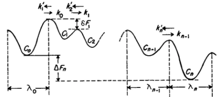
T h e succession of potential barriers over which the molecule passes is shown in Fig. 5.2 5"28 Since an actual molecular lattice is three-dimensional, we should think of the Xs as indicating the projection along the direction
24 A . Einstein, Ann. Physik [4] 17, 549 (1905); 19, 371 (1906).
2 5 Β . J. Zwolinski, H . Eyring, and C . E . Reese, J. Phys. Chem. 53, 1426 (1949).
2 6 H . Eyring, R . Lumry, and J. W . W o o d b u r y , Record Chem. Progr. 10, 100 (1949).
2 7 F. H . Johnson, H . Eyring, and M . Polissar, " T h e Kinetic Basis of Molecular B i o l o g y . " Wiley, N e w Y o r k , 1954.
2 8 R . B . Parlin and H . Eyring, in " I o n Transport Across Membranes (Η. T . Clarke, e d . ) , p . 103. Academic Press, N e w Y o r k , 1954.
(70)
102 T A I K Y U E R E E A N D H E N R Y EYRING
FIG. 5 . Free energy diagram representing diffusion in the liquid or solid state.
of the gradient of the appropriate mean j u m p distance for the molecule. If C o is the concentration of molecules per cubic centimeter at the zeroth position, then X0C0 is the number of molecules which are candidates t o j u m p across the barrier in a square centimeter of an area normal t o the direction of diffusion. T h e specific rate constant in the forward direction from the ith position is written as ki, and in the backward direction as k! ι . For the steady state we may indicate b y Q the number of molecules passing over each successive square centimeter of barriers, and write for the suc- cessive barriers the following set of equations:
Q = X o C o & o — XiCJc ι
Q = XiCiki — X2C2k'2
Q = X2C2/ c2 - X3C3/ c, 3 (71)
Q — Xn—lCn—lkn—1 XnCnk n
If we multiply the second equation above b y k\/ki, the third b y k\kf2/
( f c i f c2) , and the last equation b y k\k'2 · · · / c 'n- i / ( / c i / c2 · · · fcn_i) and add, we obtain
λ 7 In Xn k ik 2 ' ' ' k n—lk n ~ \
Ao#o I — 7 ΓΊ ; W I
\ X0 fcofci · · * fcn_i /
77 TJ-Tf TJ-p 77 \ ί Δ) 1 _|_ i L1 _ | - ^ l /c 2 _ j _ . . . _|_ ^ l fe 2 ' ' * k »-1
h kik2 kik2 - - - kn_i
Remembering that the rate constants are expressed b y equation (lb), equation (72) becomes, assuming for κ a value of unity,
Xo&0 (Co - ^ 6 ™ C n )
η = \ A° / (7<))
R E L A X A T I O N T H E O R Y O F TRANSPORT PHENOMENA 103
Here AFn is the free energy of molecules in the nth minimum minus that of those in the zeroth, and OF* is the free energy at the t o p of the barrier t o the right of the ith minimum minus that at the t o p of the barrier t o the right of the zeroth minimum.
A variety of special cases follows from equation ( 7 3 ) , and each leads t o c o m m o n l y accepted formulations of practical interest.
Case I. Suppose all barriers are of equal height; then the denominator of (73) becomes n, the total number of intervening barriers, and
= — ( a0 - a J = Po°(a0 - an)
Here, we have written δ for η λ0 , the membrane thickness, and 7 0 as the activity c o - efficient at concentration Co. D0° indicates λ ο2& ο / γ ο, and it may be called the standard diffusion coefficient. T h e quantities, ao and an are the activities at the zeroth and nth minima, respectively. T h e standard permeability P0° is defined b y
P0° = i>o°/« (75)
Case II. W e consider n o w a membrane which consists of η barriers of equal heights.
If charges of unlike sign lie on the t w o sides of the membrane with negligible net charge between, this will give rise t o a potential difference of e volts between the ze- roth and the n t h minimum. T h u s , w e have the following relations:
AFn = z g€ (76)
S F I * = (i/n)z%e (77)
o° exp ^ ~
where ζ is the valence number of the ion, g = 23,063, the faraday in units of c a l / v o l t , and k0° is the specific rate constant over the first barrier in the absence of the electric field. We write also
x = e ϋ (79)
With these substitutions, equation (73) becomes
Q = λ ο & ο ° ζ -1 /2 !
1 - I - χ + x2 + · · · - h r χ
(80)
1 /2 / Κ \
— C0x -W /2 - - Cnx-i* )
104 T A 1 K Y U E R E E A N D H E N R Y E Y R I N G Expanding the exponentials, we find that
0 £ - 1 / 2 _ xl/2 I
(81) η χ~η/2 — χη/2 n
provided that the total electrical work, z%e is somewhat smaller than RT. In this,
Thus, the transport of matter, Q, is proportional t o a permeability, Ρ = \0ko°/n. If the exponentials in equation (83) are expanded and only the first terms retained as is, of course, consistent with the approximation (81), we obtain
Thus, the total transport is the sum of a diffusion term and an electrical transport term.
In nerve membranes where e is around 80 millivolts, the expansion (81) is not always justified, and the assumption ordinarily made of an effective permeability, which is independent of voltage, should be corrected accord- ingly. In view of the popularity of expressions of the forms (83), (84), and others involving equivalent assumptions, it m a y be worthy of note to point out just how much in error such approximations may be.
W e have assumed in the a b o v e discussions that negligible net charge accumulates within the membrane, and also that the barriers are h o m o - geneous. W e will consider the properties of these assumptions. Let us as- sume that at any instant there is an excess charge in a particular " p o c k e t . "
Then, this charge in itself would cause the potential gradient to decrease automatically the driving force for transport in one direction and increase it in the reverse direction until the potential gradient as a whole is again essentially constant. W e may term this phenomenon the "incompressibility of ions" in a membrane. In a similar way, one may argue that if the mem- brane is such that there exists a priori a barrier which is much higher than those on either side, the piling up of charge at this barrier will reduce its effective height, and bring about the situation in which the sequence of barriers is very nearly a uniform one. Thus, in either case, there will be an effectively uniform succession of barriers in agreement with our assump- tions.
Using equation (80) Parlin and Eyring28 explained the establishment of the resting potential across a nerve membrane and the decay law of nerve impulse.
case,
Xok^g/n ~ \0kQ°/n = Ρ
and (83)
(84)
R E L A X A T I O N THEORY OF TRANSPORT PHENOMENA 105 It may also be pointed out that through the use of equation (80) one can also derive the expression for the liquid junction potential in accordance with those obtained b y Planck,29 H e n d e r s o n /0 and others31 b y classical treatments.
IV. Applications
In this section we give some examples showing the applications of the equations derived in the above sections. Because of the limited space for this chapter only typical examples are given. For additional examples the readers are referred to the original papers cited.
W e treat only the cases of complete equilibration of activated complexes with ambient temperature.
1. S O L I D P L A S T I C S Y S T E M
Because of the conditions given b y equations (15) to (18), the general- ized viscosity equation (34) is written as
Χιβι . χφ2 s i n h- 1 (fi2s) , x$zsmh~l (βΆέ)
η = -f- — r ( 8 ο )
Οί\ Οί2 P 2 S as ßss
I n equation ( 8 5 ) , the relations given b y (5) and ( 6 ) were introduced.
G r o u p 1, for which the condition of equation (15) holds, behaves as N e w - tonian units while other groups are non-Newtonian. G r o u p 2 for the condi- tion of equation (16) behaves differently from other non-Newtonian groups.
I t acts as N e w t o n i a n in the l o w range of shear rate, s, while it acts as non- N e w t o n i a n in the high range. I n solid plastic systems, frequently G r o u p 1 b e c o m e s n o n - N e w t o n i a n just as G r o u p 2, b u t at higher values of s. T h u s in plastics, condition (15) usually does not hold.
T h e viscosities for plastics are thus given b y the following formula:
χφι s i n h- 1 (ßie) , χφι s i n h- 1 (ß2s) χφζ s i n h- 1 (ßzs)
V = ^ h ^ h — (86)
Oil P i s Oi2 ß2s <*3 p3s
Generally, equation (85) holds for solution and for finely milled rubber, while (86) usually holds for solid systems.
E q u a t i o n (85) shows that the total viscosity η is represented b y a super- position of three curves in a plot of η vs. s, as is schematically shown in Fig. IB.
In applying equations (85) and (86), it is necessary to determine the parameters in these equations. W e consequently mention next the pro- cedures for determining these parameters.
2 9 M . Planck, Ann. Physik 39, 161 (1890) ; 40, 561 (1890).
3 0 P. Henderson, Z . Physik. Chem., 59, 118 (1907); 63, 325 (1908).
31 G . N . Lewis and L. W . Sargent, J. Am. Chem. Soc. 31, 363 (1909) ; D . A. M a c l n n e s ,
"Principle of Electrochemistry," p . 231. Reinhold, N e w Y o r k , 1939.
106 T A I K Y U E R E E A N D H E N R Y E Y R I N G
a. Determination of the Parameters
W e can resolve an experimental curve of η vs. s into its component curves using equations (85) and (86). W e mention below the procedures for this resolution in the various cases.
(1) Complete Newtonian system. T h e case where the plot of η vs. è gives a straight line which is parallel to the s-axis is the simplest case; i.e., the system behaves as a completely Newtonian system. In this case, η = χφι/αι.
(2) Non-Newtonian system without units of Group 3. In a non-Newtonian case, we first need to determine the Newtonian term, χφι/αι, b y extrapo- lating the curve of η vs. 1/s to a zero value of 1/s; for this reason, the Newtonian term is often represented b y in our papers, the oo indicating the infinite shear rate.
Using the equation
which is derived from equation (85) for the case, x% = 0, we can determine β2. T h e value of χφ<ι/α2 is the value which the quantity (η — η^) takes at s = 0. If the parameters, 77«,, , and χφι/α2, thus determined reproduce the original experimental curve in good agreement, it is concluded that the system does not have units belonging to Group 3.
(3) Non-Newtonian system with Groups 2 and 3 in addition to Group 1.
In this case, an experimental curve of 77 vs. s rises sharply in the low range of s. There are several ways to obtain curves 2 and 3 corresponding t o Groups 2 and 3, respectively, from the experimental data. T h e simplest procedure is as follows: T h e part of the experimental curve which would depend purely on Groups 1 and 2 is extrapolated to the zero value of s;
this is shown in Fig. IB b y the dotted line ab extrapolating curve 4 for large s back to s = 0.
The curve abc, so obtained, is due to the units 1 and 2. From this curve, the values of ß2 and χφι/α2 are obtained b y the same procedure as in Case (2). The contribution of Group 3 to the total viscosity is represented in Fig. IB b y the shaded area. Thus, the length of the vertical line between curves ab and db is the contribution of the flow unit of Group 3 at the value of s. Consequently, we have
the values of χφζ/αζ and β3 are calculated as before, since the values of all terms on the left side of equation (10) are known, and the value of χφ^/α^
is obtained from the value of the left side at s = 0.
(4) Non-Newtonian system without Newtonian Group. In some cases, the V — χφ2 sinh 1 ß2s
a2 ß2s (87)
(88)
R E L A X A T I O N T H E O R Y OF T R A N S P O R T P H E N O M E N A 107 extrapolation of the curve η vs. l/s t o the zero of 1/s gives an extremely
small value. This is the evidence for the absence of the Group 1, Newtonian units. E v e n in this case, the experimental curve in the lower range of s is well fitted b y equation (87) for Case (2), a system composed of N e w - tonian units and non-Newtonian units of Group 2. This illustrates the fact that the Newtonian units became non-Newtonian in the higher range of s.
Assuming there is no Group 3, the viscosity formula in this case is de- rived from equation (86) as follows:
Xißi s i n n- 1 βιέ x2ß2 s i n h- 1 ß2s ,οπΝ
V = + (89) Oil ßlS
0>2
P 2 SF r o m equation (89) one obtains the equation
/ = ^} s
+ Ξ! in 2s + - In ft (90)on a2 OÎ2
where equation (5) and the relation
s i n h- 1 ß2s In 2ß2e (91)
are introduced into equation ( 8 9 ) . Equation (91) holds only for large values of s, while equation (5) holds for small values of è. T h a t is, the t w o paradoxical relations are introduced into the same equation, equation (86).
Although equation (90) thus m a y seem illogical, it is in fact very useful in determining the approximate values for the parameters, χφι/αι, x2/a2, and ß2 in equation ( 8 9 ) . T h e s e a p p r o x i m a t e values are then introduced in equation (87) t o make it fit the experimental curve in the l o w range of s.
Using the best values for the parameters, the viscosity η' is calculated from equation (87) for the whole range of s. T h e value of η' deviates in the high range of è from the experimental η which fits equation (89). F r o m equations (87) and (89), the deviation η' — η m a y be written
- , = gift
(
1 - s i n lf **)
(92)« i \ pis /
The value of βι can n o w be calculated, since Χ\β\/α\ is already known.
Applying the principles previously outlined, one can determine the parameters in the case where three non-Newtonian units are present [see equation (86)]. T h e details will not be given here.
b. Results
(1) Natural rubber. Saunders and Treloar32 obtained s vs. / curves for
32 D . W. Saunders and L. R . G. Treloar, Trans. Inst. Rubber Ind. 24, 92 (1948); L . R . G . Treloar, " T h e Physics of R u b b e r E l a s t i c i t y , " p . 198. Oxford Univ. Press, N e w Y o r k , 1949.
108 T A I K Y U E R E E A N D H E N R Y E Y R I N G
5 5 log f(dynes/cm2)
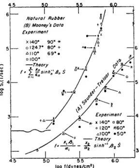
FIG. 6. Logarithm of reduced shear rate vs. logarithm of shear stress for masticated rubber. T h e data of Saunder and Treloar (see ref. 32) are referred to the right and b o t t o m coordinates while M o o n e y ' s data (see ref. 33) are referred to the left and upper coordinates. T o avoid the complexity caused b y the superposition of many data around the same point, the following procedure was adopted in this figure: T h o s e data which could not be plotted in their real position, because of the superposition, were put outside the points, and arrows were used to show where the data belonged.
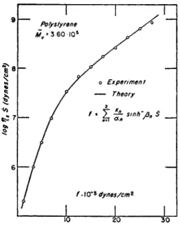
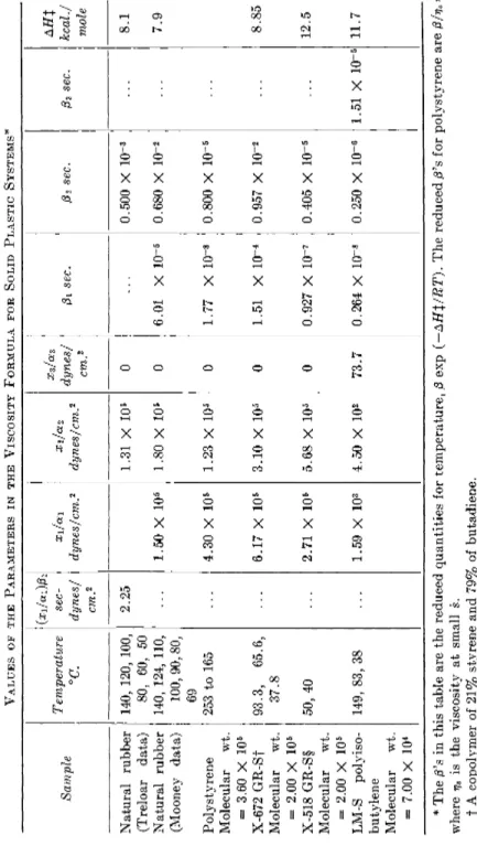
masticated rubber at temperatures form 50 to 140° C. T h e y found that the so-called Ostwald-de Waele equation, s = kfn (k and η are constant), does not adequately represent their curves. T h e y found also that the activation heat for the flow process was 8.1 kcal./mole. W e calculate a reduced shear rate, s exp (AHX/RT), from their curves using their activation heat; the logarithms of the reduced shear rates sr are plotted against log / i n Fig. 6 A . W e see that the reduced rates calculated from the data at various tem- peratures agree very well except at 50° C. T h e deviation of the data at 50° C. m a y be due to some second-order transition which takes place around this temperature.3 2a T h e full curve was obtained b y calculation from equation (87), using the values of the parameters in Table I, where the parameters for other samples are also summarized. W e see that the
3 2a If this is true, this transition is different from that which takes place at —73° C*
See H . Mark and Α . V . T o b o l s k y , "Physical Chemistry of High Polymeric Sys- t e m s , " p . 346. Interscience, N e w Y o r k , 1950.