ANALYSIS OF TRIBOLOGICAL PHENOMENA IN VISCOUS FLUID FLOWS OVER SOLID SURFACES

(1)

ANALYSIS OF TRIBOLOGICAL PHENOMENA IN VISCOUS FLUID FLOWS OVER SOLID SURFACES

by

Gabriella Vadászné Bognár

University of Miskolc

Faculty of Mechanical Engineering and Informatics

Submitted for the degree of

“Doctor of the Hungarian Academy of Sciences”

Category:

“Technical Science”

(2)

1 Introduction

In the 1800s, applying the basic principles of mass conservation and Newton’s second law, Leonhard Euler described the fluid flow in terms of spatially vary- ing three-dimensional pressure and velocity fields by two coupled nonlinear partial differential equations. Euler did not account for the effect of friction acting on the motion of the fluid elements. In 1822 Claude-Luis Navier [158]

and independently in 1845 George Stokes [192] took the viscous forces into considerations and derived the mathematical description of a viscous fluid flow by a system of more complex nonlinear partial differential equations called Navier-Stokes equations. No one has given a general analytic solution to them. In 1904 Ludwig Prandtl introduced the concept of the boundary layer in a fluid flow. From that time the modern aerodynamics and fluid dynamics have been dominated by Prandtl’s idea. Prandtl has given the first description of the boundary layer concept in his paper [168] entitled ” ¨Uber Fl¨ussigkeitsbewegung bei sehr kleiner Reibung” (”On the motion of fluids with very little friction”). In his theory an effect of friction was to cause the fluid adjacent to the solid surface to stick to the solid surface of the body submerged in the fluid flow (i.e., no-slip condition at the surface) and the frictional effect was experienced in a thin region near the surface. That boundary layer is very thin in comparison with the size of the body of the object. Prandtl concluded that if the viscosity is small, the velocity changes substantially in a very short distance normal to the solid surface. Within the boundary layer the velocity gradient is very large. With the Newton’s shear-stress law (i.e. the shear stress is proportional to the velocity gradient and viscosity) the local shear stress can also be very large. Near the solid surface in the thin boundary layer the friction is dominant while in the outer inviscid flow external to the boundary layer the friction is negligible. The outer flow generates the boundary conditions at the edge of the layer.

With Prandtl’s idea it became available to reduce the Navier-Stokes equations to differential equations of simpler form called boundary layer equations [13]. While the Navier-Stokes equations are elliptic and the complete flow field must be solved simultaneously, the boundary layer equations are parabolic for which simplifications are available (see e.g., [10], [13], [74], [76], [177], [178]). In 1908 Heinrich Blasius [30] gave solutions for two-dimensional boundary layer flows over a flat plate and a circular cylinder. For constant pressure along the flat plate oriented parallel to the flow, the coupled nonlinear partial differential equations were reduced to a nonlinear ordinary differential equation called Blasius equation [30].

In 1921 von K´arm´an [119] and Pohlhausen [165] provided an approximate method, which has been used with considerable success for the analysis of

(7)

boundary layer flows. The method is based on an integral formulation of the problem and its result, the calculated flow field, usually satisfies the equations of continuity and momentum. The boundary conditions for the flow are expanded to polynomial functions as an approach for the velocity profiles in the laminar boundary layer.

Exact solutions to problems involving the motion of fluids are very dif- ficult, or even impossible to obtain, even when the geometry is simple and the fluid’s physical properties are constant. Numerical solutions are usually good options but, when an analytical description is required, approximate methods of formulation and solution are often useful.

1.1 Lubrication and Materials Processing

Lubrication, spreading, polymer coating and processing, and thin film casting are important applications of the flow near a solid wall in engineering. Com- putational analysis of flow near solid surfaces is performed to complement the experimental observations. The advantage of the theoretical investigations over experiments is that one can control the conditions and parameters in the analyzed problem to predict velocity profiles and shear stress, and it can be used also for assessing the error of numerical simulations of the problem.

The first paper on fluid-film lubrication of journal bearings was published in 1883. The hydrodynamic effect has been shown experimentally by Tower [204]. In 1886, Reynolds developed on the base of Tower’s results his theory of hydrodynamic lubrication by assuming the fluid as viscous and Newto- nian. However, in real situations, non-Newtonian fluids are used in order to increase the viscosity of the lubricants by adding additives to base oils. The addition of polymers to mineral oils has spread in practice [198], [24]. To predict the mechanical behavior of these lubricants is much more complicated than of mineral oil lubricants which are considered Newtonian fluids. The resulting lubricants, e.g., silicone fluids and polymer solutions are described by non-Newtonian power-law model due to the model’s simplicity ([154], [181], [182], [183], [184]. The non-Newtonian lubricants are encountered in various processes of lubrication. Recently, considerable effect has been expanded for solving problems in tribology regarding the non-Newtonian influence on lubrication flow characteristics of squeeze films ([154], [181], [182]), externally pressured bearings ([183], [184]), journal bearings ([198], [173], [211]) and roller bearings ([186], [187]).

Because of the importance of tribology and materials processing, considerable research effort has been directed at the transport phenomena in such processes in recent years. Many books are available on the area of lubrication, manufacturing and materials processing (see e.g., [9], [75], [87], [108], [126],

(8)

[149], [145], [195], [196], [198]). Fluids engineering research can impact on the field of tribology and materials processing only if significant effort is also directed at understanding the basic mechanisms. In the last four decades the demand in materials processing of composites, ceramics and advanced polymers has been increasing.

An intense research of fluid flow mechanism arising in many materials processing applications is necessitated to improve product quality, reduce costs and achieve custom-made material properties. Fluid flow appears in a lot of material processing operations e.g., in crystal growth for semiconductor fabrication, polymer extrusion, casting or continuous processing of thin films.

Due to the importance of fluid flow in materials processing, extensive research is being done in this field. Jaluria [117] gave a review on the main aspects that must be considered in material processing, on the fluid flow phenomena involved in different areas, such as drying, heat treatments, metal forming, casting, crystal growing, polymer extrusion, food processing, coating and microgravity materials processing. He emphasized that relatively little information can be found in the literature on the link between the diverse processing techniques and the basic mechanisms of the govern flow; and the quantitative dependence of the product quality on the fluid flow. Fluid flow properties are important in many manufacturing processes as they effect on the transport mechanisms, on the impurities and defects, on the time spent by the material in the system, on the properties and characteristics of the final product and on the product quality [209]. It is important to understand the basic flow mechanisms involved in these processes so that high quality coatings can be achieved at relatively large speeds of the coated material (see Kistler and Schweizer [122] ). The casting processes have been reviewed by Ruschak [172]. Weinstein and Ruschak [209] have pointed out that predictive analysis is usually not available for the coating methods. Therefore, it is ad- vantageous to describe the mechanical details for the fluid flow components and then combine this knowledge for the applications. The main interest is the achievable coating thickness and the uniformity, the attainable speed together with the rheological requirements.

The production and use of polymers have grown increasingly. The extrusion process is one of the most important polymer processing techniques today. The extruders produce a tremendous variety of products. For example, in the plasticating extruder the solid polymer is melted, homogenized and pumped through the die at high pressure and temperature (see and [27], [87], [149], [153]).

The processing of sheet-like materials is a necessary operation in the production of paper, linoleum, polymeric sheets, roofing shingles, insulating materials, and fine-fiber matts. Virtually, in all such processing operations,

(9)

the sheet moves parallel to its own plane [9]. The moving sheet may induce motion in the neighboring fluid or, alternatively, the fluid may have an independent forced-convection motion that is parallel to that of the sheet.

1.2 The Basic Equations in Rectangular Coordi- nate System

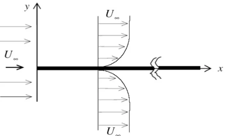
We shall consider laminar fluid flows with constant densityρ over a thin flat plate in a uniform stream with velocity U∞. The kinematic and dynamic viscosity are denoted by ν and µ, respectively. Consider the plate of length L. We assume that the Reynolds number Re = ρU_∞L/µ expressing the quotient from inertial and viscous forces is small, the flows considered in this study are laminar. The fluid flows in parallel layers next to the solid surface.

Fig. 1.1 Boundary layer flow along a plate

The x >0 and y >0 are the Cartesian coordinates along and normal to the plate with y= 0 is the plate and the coordinate xis as taken positive in the direction of the mainstream. The plate origin is located at x = y = 0, and u, v represent the components of the fluid velocity in the direction of increasing x and y, respectively (see Fig. 1.3).

The governing equations for fluid flow and the associated heat transfer in materials processing are derived from the basic conservation principles for mass, momentum and energy. The continuity equation for an incompressible fluid can be formulated as

(1.1) ∂u

∂x +∂v

∂y = 0.

(10)

The equation of motion is a vectorial equation. For steady, a two- dimensional fluid flow it can be formulated under the assumptions that the flow is independent of time, laminar and the gravity forces are neglected [26], [149], [210]:

ρ(u∂u

∂x +v∂u

∂y) = −∂p

∂x +

∂τ_xx

∂x +∂τ_yx

∂y

, (1.2)

ρ(u∂v

∂x +v∂v

∂y) = −∂p

∂y + ∂τ_xy

∂x + ∂τ_yy

∂y

, (1.3)

where τxx, τyy, τxy, τyx are the components of the stress tensor.

Taking into consideration the components of the stress tensor in rectangular coordinates [26] equations (1.2) and (1.3) are reduced to

ρ

u∂u

∂x +v∂u

∂y

= −∂p

∂x + 2 ∂

∂x

(µ∂u

∂x)

+ ∂

∂y

µ(∂u

∂y + ∂v

∂x)

, (1.4)

ρ

u∂v

∂x +v∂v

∂y

= −∂p

∂y + ∂

∂x

µ(∂u

∂y +∂v

∂x)

+ 2 ∂

∂y

(µ∂v

∂y)

, (1.5)

where µdenotes dynamic viscosity.

The velocity in the boundary layer increases until it reaches the outer flow velocity U∞. As all fluid flows must be zero at a solid boundary, the velocity must increase rapidly to U∞ in a boundary layer. The region of velocity change is called a hydrodynamic boundary layer . The boundary layer thickness δbl is defined as the distance required for the flow to reach U∞.

Prandtl’s boundary layer theory applies to flows where there are extensive inviscid regions separated by thin shear layers of boundary layer thickness δ_bl L. It is satisfied if Re 1. Except this close neighborhood of the solid surface, the flow velocity is comparable to the free stream velocity U∞. Outside the boundary layer the velocity gradients are negligibly small and the influence of the viscosity is unimportant. In the flow of the region near the solid surface there is friction. In the normal direction y inside the thin layer the gradient ∂u/∂y is very large compared with gradients in the streamwise direction ∂u/∂x. Although the viscosity was meant to be very small in this flow, the shear stress can be large. For steady flows the approximations used by Prandtl (1904) in deriving the boundary layer equations are the following:

Re1, δbl L, v u, ∂u/∂x ∂u/∂y, ∂v/∂x ∂v/∂y.

moreover, ∂p/∂y≈ 0, thenp=p(x) only, and if the free stream outside the boundary layer is U∞(x), then

∂p

∂x =−ρU∞

dU∞

dx .

(11)

Within the framework of these assumptions the governing equations of motion (1.2) and (1.3) for a flow of constant property fluid neglecting the buoyancy and the body forces can be substituted by ([171], [178], [225]):

(1.6) ρ

u∂u

∂x +v∂u

∂y

=ρU∞

dU_∞

dx +∂τ_yx

∂y .

If the temperature of the wall is different from that of the free stream, there is a thermal boundary layer thickness different from the flow boundary layer thickness. To predict the temperature variation we need an equation for the temperature field in the boundary layer.

The equation of energy for a steady two-dimensional boundary layer without heat sources in rectangular coordinates takes the form ([171], [178], [201], [202], [225]):

(1.7) u∂T

∂x +v∂T

∂y = ∂

∂y

α_t∂T

∂y

,

where T is the temperature of the fluid in the boundary layer and α_t is the thermal diffusivity. Equation (1.7) includes the following approximations i.) the pressure variations in the flow are not enough to affect the thermodynamic properties,

ii.) the viscous stresses do not dissipate enough energy to warm the fluid significantly and

iii.) in the boundary layer ∂²T /∂x² ∂²T /∂y².

It should be noted that the boundary layer equations are not exact but are asymptotic forms of the basic hydrodynamic equations when the Reynolds number is large. The experimental flows at large Reynolds numbers are turbulent, yet useful comparisons with laminar flow experiments at moderate large Reynolds numbers can sometimes be made with large Reynolds number asymptotic theories [71]. We restrict ourself for studying only the laminar boundary layer flow.

In the following sections we study the possibility of reducing the system of equations (1.1), (1.6) and (1.7) to ordinary differential equations by similarity transformation. The term ”similarity solution” in fluid mechanics was first introduced by Blasius [30] when he found a solution to a problem of Prandtl’s boundary layer theory. Generally, a similarity solution is one in which the number of variables can be reduced by some analytical techniques, e.g. by a coordinate transformation. The theory of similarity in physical problems has been investigated in several books from mathematical approaches by Ames [10], or from physical viewpoint by Sedov [180] and Hansen [99].

The similarity method is a technique which reduces a set of partial differential equations into ordinary differential equation(s) involving only a single

(12)

variable. A systematic approach to provide solutions to partial differential equations by the solution of ordinary differential equations which were obtained by special transformations of the dependent/independent variables.

It is the use of specific combinations of variables which enables a conversion of the partial differential equation to an ordinary differential equation.

Similarity analysis is applicable to certain problems in which the characteristic lengths are determined by rate processes rather than by the geomet- ric or physical dimensions. Such problems generally involve regions which are regarded as being semi-infinite. The field variable of velocity attained through similarity method has profiles which are identical in shape for all positions or times, differing only by the scale over which the variations occur and described by a variable of similarity. The benefit of the similarity analysis is that a set of partial differential equations can be reduced to ordinary differential equations. This mathematical gain is accompanied by a loss in generality. Similarity solutions are limited to certain geometries and certain boundary conditions.

In sum, a primary advantage of the similarity method is that it is one of the few general techniques for obtaining exact (nonlinear) solutions of partial differential equations. A primary disadvantage of the similarity method is that the solution found may satisfy only a very restricted set of initial and boundary conditions.

1.3 Boundary Conditions

We must specify the boundary conditions to the set of differential equations (1.1), (1.6) and (1.7). Many of the boundary conditions are the usual no- slip conditions for velocity and the appropriate thermal or mass transfer conditions at the boundaries. In general, boundary conditions are divided into three types: initial conditions, surface boundary conditions and field boundary conditions.

Initial conditions are specified at an initial position on the surfaces, e.g.

at the leading edge of a semi-infinite flat plate.

Surface boundary conditions are specified at the solid surface of the body.

Usually, it gives conditions on the velocity components and on the temperature or heat transfer rate at the surface. The no-slip condition means that the velocity of the fluid at the solid surface is assumed equal to the velocity of the surface. Similarly, the temperature of the fluid at the solid surface is assumed equal to the surface temperature. Instead of giving the temperature at the surface, the heat transfer rate can also be given, i.e., the temperature gradient at the solid surface can be specified. Surface tension effects are important in many materials processing flows. Examples include flows in

(13)

welding, Czochralski and the floating-zone crystal growing methods, wave soldering, and continuous casting. Surface tension can also have a significant effect on the flow near the free surface. Large surface tension gradients can arise along the interface due to temperature and concentration gradients.

Such surface tension gradients can generate significant shear stresses and resulting flow along the interface. This flow, known as thermocapillary or Marangoni convection, is important in many material processing flows [126].

Furthermore, the mass flow rate through the surface can be specified. If the mass flow rate through the surface is zero the velocity component normal to the surface is zero. Positive mass flow rates are referred to as blowing or injection and negative mass flow rates as suction.

The field boundary conditions are given at some point in the flow field usually at a large distance from the surface. The velocity components and/or thermodynamic variables can be required to approach a constant or some specific functional form.

1.4 Viscosity Variation

The properties of the material undergoing thermal processing play a very important role in the mathematical and numerical modeling of the process.

The variation of dynamic viscosity µ requires special consideration for materials such as lubricants, plastics, polymers, food materials and several oils, that are of interest in a variety of manufacturing processes. Most of these materials are non-Newtonian in behavior, implying that the shear stress is not proportional to the shear rate. The viscosityµis a function of the shear rate. For Newtonian fluids like air and water, the viscosity is independent of the shear rate, but increases or decreases with the shear rate for shear thickening or thinning fluids, respectively. These are viscoinelastic fluids, which may be time-independent or time-dependent.

The mechanical behavior of a material and its mechanical or rheological properties can be characterized in terms how the shear stress and shear rate are related. If the properties of the fluid are such that the shear stress and shear rate are proportional, the material is known as aNewtonian fluid. This relationship in the boundary layer is expressed by

(1.8) τ_yx =µ∂u

∂y

called Newton’s law of viscosity. For materials which do not obey this law, i.e., the shear stress and shear rate are not directly proportional but are related by some function, the fluid is called non-Newtonian [213]. Many of industrial liquids show non-Newtonian behavior, see for example [22],

(14)

[27]-[29], [213]. The physical origin of a non-Newtonian behavior relates to the microstructure of the material. Materials such as slurries, pastes, gels, drilling mud, paints, foams, polymer melts or solutions are examples of non- Newtonian fluids. For such fluids the viscosity is not constant, it is a function of either the shear rate or the shear stress.

Many papers have concentrated on the prediction of rheological properties under shear using molecular dynamics computations ([89], [90], [226]).

The observations of these simulations greatly assist us in understanding the behavior of lubricant properties. Various models are employed to represent the viscous or rheological behavior of fluids of practical interest. Frequently, the fluid is treated with the non-Newtonian viscosity function given in terms of the shear rate.

A chief difficulty in the theoretical study of non-Newtonian fluid mechanics is to define this relationship. The apparent viscosity µ_app is the ratio of shear stress and shear rate, then

τ_yx =µ_app∂u

∂y

holds. We shall investigate boundary layer problems for non-Newtonian fluids whose apparent viscosity depends only on the rate of strain. The actual mathematical form of µapp for these materials will depend on the nature of the particular material. The flow behavior of fluids determined by their rheological properties is described by the relationship between the shear stress and shear rate. This relationship is determined experimentally. The time- independent viscoinelastic fluids are often represented by

(1.9) µ_app =K φ

∂u

∂y

, where φ is an empirically determined function.

The most common flow model is the so-called power-law model or the Ostwald-de Waele power-law model, given by [195]. Throughout this work we apply this model when the flow behavior of the non-Newtonian fluid is described by

(1.10) µapp =K

∂u

∂y

n−1

.

This provides an adequate representation of many non-Newtonian fluids over the most important range of shear. The shear stress is related to the strain rate ∂u/∂y by the expression

(1.11) τ_yx=K

∂u

∂y

n−1 ∂u

∂y,

(15)

whereK andn >0 are a positive constants called consistency and power-law index, respectively, and defined by Bird [26]. The case 0 < n <1 corresponds to pseudoplastic fluids (or shear-thinning fluids), the case n > 1 is known as dilatant or shear-thickening fluids. For n = 1, one recovers a Newtonian fluid. The deviation ofn from a unity indicates the degree of deviation from Newtonian behavior [13].

It should be noted that without the above boundary layer simplifications the dynamic viscosity µ in (1.4) and (1.5) for power-law fluids is calculated by the following relationship

(1.12) µ=K

( 2

"

∂u

∂x 2

+ ∂v

∂y 2#

+ ∂u

∂y + ∂v

∂x

2)(n−1)/2

.

The two-parameter relations (1.11) or (1.12) have been useful in fitting rheological data for a large variety of fluids (see [153], [179]). Parameters K and n are determined empirically. Relation (1.11) may fail to fit the total range of experimental data for some materials. However, the formula can be fitted well to measured data over a restricted range of shear rate. The properties of the material undergoing thermal processing must be known and appropriately modeled to accurately predict the resulting flow and transport, as well as the characteristics of the final product. Some of the values of n are shown in Table 1.1 ([57], [63], [161]). In process industries most non- Newtonian fluids are pseudoplastic (n <1).

The ”functionalization” of solid and fluid materials by addition of chem- ical compound is a process that is going back to Maxwell [147], [148] and Rayleigh [170]. The effective viscosity was characterized by Einstein [80], [81]. Due to measurements for crude oil and experiments with various liquids ranging from simple molecular liquids to polymer melts it was shown that the apparent viscosity dependent on the shear rate. On the base of measurements the authors observed for the apparent viscosity a power law of the form (1.10). The dependence of the powern on many factors (e.g. the pressure, the temperature and the film thickness) was confirmed by simulations ([2], [133], [134], [79]). Application of molecular dynamics to rheology has helped to understand the behavior of non-Newtonian fluids to predict quantitative rheological properties such as the viscosity of lubricants [116].

Some lubricants, e.g. silicone fluids and polymer solutions are described by the non-Newtonian power-law model due to the model’s simplicity (see [154], [181], [182], [183], [184]).

(16)

Material n

clay suspension 0.1

suspensions (kaolin in water, bentonite in water) ≈0.1-0.15

cosmetic cream ≈0.1-0.4

toothpaste 0.3

molten polymers ≈0.3-0.7

drilling fluid (oil based mud), paper pulp, latex paint ≈0.4-0.6

lubricants ≈0.4-1.1

water, glycerin 1

slurry (sand-water mixture) ≈1.1-1.4

saturated honey ≈1.5

Table 1.1

Thompson et al. [199] showed that at high shear rates the viscosity of glassy films obeys a power law in the form (1.10) with n = 2/3. In [41] and [52] the power exponent n was determined for a polyethylene and n ≈0.3 was obtained in the range of temperature 160^◦C-180^◦C. It was shown that both K and n depend on the temperature. In case of sand-bentonite- water mixtures for different sand volumetric concentrations the experiments gave n ≈ 1.4 and here the rheological parameters K, n do depend on the volumetric concentration [49].

For simplicity, in our calculations we assume that the power-law exponent n and the consistency K are constants. Even if the main advantage of the power-law model is its relative simplicity, the non-Newtonian behavior of the material complicates the viscous terms in the momentum equation.

Remark. Due to the wide range of applications a large number of ar- ticles has been devoted to different mathematical aspects of the so-called p- Laplacian operator ∆_pu =∇(|∇u|^p−2∇u). Here, instead n the p parameter is applied. On the mathematical examinations of the solutions to the equations involving ∆p we mention the book by Doˇslý and Rehák [77], Drábek and Milota [78] and also some of my papers [31]-[37]. That type of nonlin- earity appears also in nonlinear diffusion equations arising from a variety of diffusion phenomena ([36], [216]).

1.5 Investigations

Analytical and numerical techniques can be applied to investigate flow characteristics and how the fluid flow affects the process and the product. In general, predictive modeling of complex processes is not yet known. The practice remains largely empirical. However, physical insights and mathematical models are greatly beneficial to explore the effect of the fluid flow on

(17)

the lubricated machine elements or on the final product. Due to the practical necessity, it is important to study the influence of the viscosity on the lubrication velocity and temperature fields. Within the thin boundary layer, the wall shear stress and the friction drag of the solid surface can also be esti- mated. It is important to understand the fluid flow mechanisms determined by the governing equations and boundary conditions along with important parameters to minimize and control their effects.

Due to the complexity of the governing equations and boundary conditions that analytical methods can be used to obtain the solution in very few practical circumstances. However, numerical approaches are extensively used to obtain the flow characteristics, analytical solutions are very valuable since they can be used for verifying numerical models, they provide information about the basic mechanisms and give quantitative results for some components. Analytical solutions can be obtained for simplified and idealized models of certain processes.

The main topic of this dissertation is to introduce, review and discuss several models which can be investigated by similarity analysis. Our results are given for some boundary layer problems of Newtonian or non-Newtonian fluid flows over horizontal solid surfaces.

In Section 2.1, the boundary layer problem for an idealized Newtonian viscous fluid past a semi-infinite flat plate is one of the best known problems in fluid mechanics, as its first analytic solution for the laminar case dates back to the beginning of the last century with Blasius [30]. The classic book by Schlichting and Gersten [177] describes the similarity approach of Newtonian fluid flow problem called the Blasius problem. The similarity solution and T¨opfer’s transformation [203] are reviewed.

The first analysis of the boundary-layer equations for a power-law fluid is due to Schowalter [179] and Acrivos et al. [4] in 1960. In Section 2.2, we deal with the analysis of similarity solutions of the two-dimensional boundary layer flow of a power-law non-Newtonian fluid past a semi-infinite flat plate.

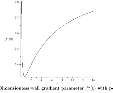
The boundary value problem of the momentum equation is converted into initial value problem by applying proper similarity variables and the partial differential equations are transformed into the so called generalized Blasius equation. For this we apply a T¨opfer-like transformation to determine the dimensionless wall gradient numerically. The power series expansion of the solution is also presented for n >0 ([38], [47]).

In Section 2.3, the similarity solutions to the Prandtl boundary layer equations describing a non-Newtonian power law fluid past an impermeable flat plate, driven by a power law velocity profile U_e = ˜By^σ ( ˜B > 0) are investigated. We give that there are analytical solutions for any n >0, n 6= 2 and any−1/2≤σ < 0 and examine the effect of parametersσ, andn on the

(18)

velocity profiles [46].

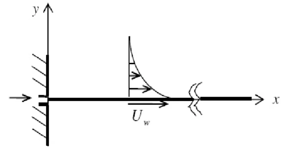
Boundary layer behavior on a moving continuous solid surface occurs in a number of materials processes, an example is a polymer sheet or filament extruded continuously from a die. The flow behavior was theoretically studied by Sakiadis [175] and experimentally by Tsou et al. [205]. Since some polymers are flexible materials, the filament surface may stretch during the production and therefore the surface velocity deviates from being uniform.

Sakiadis studied the flow induced by the uniform motion of a continuous solid surface. Crane [72] gave an exact boundary layer solution, which is an exact solution of the Navier-Stokes equations, for continuous sheet when the sheet velocity is proportional to distance from the extrusion origin. In Section 3.1, the boundary layer equations are considered for two-dimensional boundary layer flows of Newtonian fluids over a moving flat surface moving at a speed of U_w(x) in an otherwise quiescent Newtonian fluid medium. We give a generalization of Crane’s solution for stretching wall with power law stretching velocity [43]. The shear stress at the solid surface and the interval of convergence are also discussed.

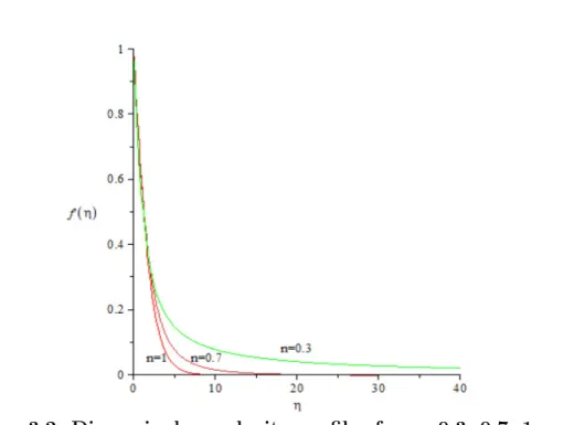
A technologically important source of the boundary layer phenomenon is the non-Newtonian fluid flow over a continuously moving solid surface. For example, hot rolling, glass-fiber production and conveyor belt are included in the applications. In Section 3.2 we provide a theoretical analysis of the boundary layer flow on a flat solid surface moving in an otherwise quiescent non-Newtonian fluid medium. A special emphasis is given to the formulation of boundary layer equations, which provide similarity solutions for the velocity profiles. We give numerical results on the velocity profiles and represent the effect of the power exponent on the shape of the velocity distribution [39].

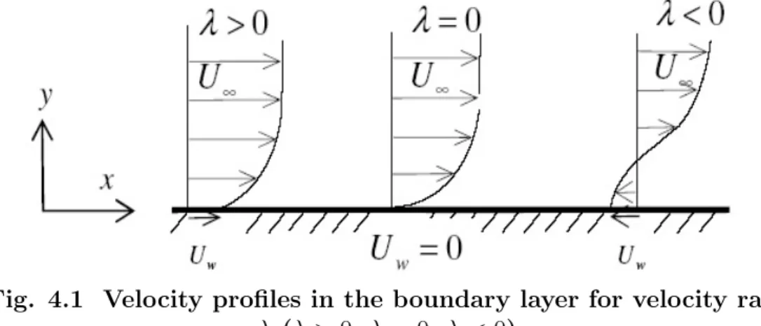
After Blasius’ pioneering work in 1908, more than three decades later the uniqueness of Blasius’ famous velocity boundary layer solution was rigor- ously proved by Weyl [212]. On this background it was quite surprising that further three decades later, Steinheuer [191] and Klemp and Acrivos [123], [124] reported that in the Blasius-problem non-unique solutions may occur when the plate is not at rest, but moves with a constant velocity U_w, opposite in direction to the free stream of velocity U_∞. It means that for positive values of the velocity ratio λ = −U_w/U∞ dual solutions exist as long as λ is smaller than the critical value λ_c = 0.3541. . . , after which no similarity solutions exist. For λ < 0, Callegari and Nachman [62] have found unique solutions. The aim of Section 4.1 is to give an introduction to the results on the development of the doubly-driven Blasius flows reported by Klemp and Acrivos in their Journal of Fluid Mechanics papers [123], [124] and by Steinheuer [191]. In Section 4.2, our purpose is to give a theoretical analysis

(19)

of similarity solutions for the boundary layer of a non-Newtonian fluid on a flat plate moving opposite to the stream. The generalized Blasius boundary value problem is considered with non-homogeneous lower boundary conditions f(0) = 0, f⁰(0) = −λ, where λ is the velocity ratio. The numerical calculations indicate that for non-Newtonian fluids there is a critical value λ_c such that solution to the boundary layer problem exists only if λ < λ_c. For Newtonian fluid (n = 1) this phenomena was shown by Hussaini and Lakin [110] and λ_c was found to be 0.3541. . . . We give estimation analyti- cally for the critical velocity ratio λ_c depending on the power-law exponent n and show the dependence of λ_c on the power exponentn [44].

When a free liquid surface is present, the surface tension variation resulting from the temperature gradient along the surface can also induce motion in the fluid called thermal Marangoni convection. Marangoni convection is mass transfer along a liquid surface and it appears in many engineering problems. e.g., in highly stressed lubricated ball or friction bearings [125], and in crystal growth melts [67]. These phenomena have also been investigated by similarity analysis (see [14], [16], [65]-[67], [164]). In Section 5.1, we present the derivation of the equations and show how the boundary layer approximation leads to the two points boundary value problem and the similarity solutions for Newtonian fluids. The new model, written in terms of stream function and temperature, consists of two strongly coupled ordinary differential equations. Its analytical approximate solutions are represented in terms of exponential series. The influence of various physical parameters on the flow and heat transfer characteristics are discussed [48].

Many principal past studies concerning natural convection flows over a semi-infinite vertical plate immersed in an ambient fluid have been found in the literature ([141], [225]). In many cases, these problems may admit similarity solutions. The idea of using a convective boundary condition for New- tonian fluids was recently introduced by Aziz [18], while Magyari [143] revis- ited this work, and obtained an exact solution for the temperature boundary layer in a compact integral form. The effects of suction and injection have been studied by the similarity analysis by Ishak [115] and a couple of recent papers have been devoted to the subject of boundary layer flow with convective boundary conditions (see e.g., [11], [45], [97], [100], [101], [144], [162], [169], [193], [194], [217], [218]). Motivated by the above mentioned studies, in Section 5.2 we investigate the steady laminar boundary layer flow of a non- Newtonian fluid over a permeable flat plate in a uniform free stream, when the bottom surface of the plate is heated by convection from a hot fluid. We examine the heat and velocity distributions of a viscous and incompressible power-law non-Newtonian fluid over a permeable steady sheet in a uniform shear flow with a convective surface boundary condition ([45], [50]).

(20)

2 Boundary layer flow on a flat plate

The simplest example of application of boundary layer equations is the fluid flow along a stationary solid surface. Although experimental studies of such flows are important, it is crucial that the fluid mechanical properties are determined. Theoretical understanding of the flow behavior is necessary. We predict the boundary layer flow field by solving the equations that express conservation of mass and momentum in the boundary layer for Newtonian and non-Newtonian media. The geometry allows the governing partial differential equations to be reduced to ordinary differential equations using a similarity transformation.

2.1 Newtonian fluid flow

The problem of Newtonian fluid flow along a stationary, horizontal, infinite, plate situated in a fluid stream moving with constant velocityU∞is a classical problem of fluid mechanics. In this problem, the fluid motion is produced by the free stream. The Blasius flow is the result of the interaction of a flow that is spatially uniform for large x with a solid plate, which is idealized as being infinitely thin and extending infinitely far to the right as x → ∞.

The simplifications in the Navier-Stokes equations are valid for very high Reynolds numbers

(2.1) Re = ρU∞L

µ .

Although the geometry is idealized, all flows past a solid body have thin boundary layers similar to the Blasius flow. Air rushing past a bird or an airplane, ocean currents streaming past an undersea mountain - all have boundary layers. The Blasius problem has developed a vast bibliography with the most well-known book written by Schlichting and Gersten [177].

2.1.1 Basic equations

We review the steady-state classical problem of a fluid flow along a horizontal, stationary surface located in a uniform free stream U_∞. This problem has been solved first by Blasius [30].

Let us consider the boundary layer governing equations (1.1), (1.6) for the two-dimensional steady flow of an incompressible fluid parallel to the x axis (see Fig. 2.1). In this case the velocity of the potential flow is constant, and

∂p/∂x= 0. For Newtonian fluids the shear stress and shear rate relationship

(21)

Fig. 2.1 Boundary layer on a flat surface at zero incidence

given by (1.8). The boundary layer equations (1.1) and (1.6) become

∂u

∂x + ∂v

∂y = 0, (2.2)

ρ

u∂u

∂x +v∂u

∂y

= µ∂²u

∂y². (2.3)

To solve these equations three boundary conditions are needed:

(i.) at the solid surface there is neither slip nor mass transfer:

(2.4) u(x,0) = 0, v(x,0) = 0,

(ii.) outside the viscous boundary layer the streamwise velocity component u should approach the main stream velocity U∞:

(2.5) lim

y→∞u(x, y) = U∞. 2.1.2 Similarity solution

In order to study this problem it is convenient to introduce the stream function ψ defined by

(2.6) u= ∂ψ

∂y, v =−∂ψ

∂x.

Then, the continuity equation (2.2) is satisfied automatically and the equation (2.3) becomes

(2.7) ∂ψ

∂y

∂²ψ

∂y∂x − ∂ψ

∂x

∂²ψ

∂y² =µ_c∂³ψ

∂y³, µ_c=µ/ρ.

(22)

The boundary conditions (2.4), (2.5) can be written as

∂ψ

∂y (x,0) = 0, ∂ψ

∂x (x,0) = 0, lim

y→∞

∂ψ

∂y (x,0) =U∞.

Now, we have a single unknown functionψ in the partial differential equation (2.7). We look for similarity solutions using the linear transformation x → ωx, y → ω^−βy, ψ → ω^−αψ with a positive parameter ω. Equation (2.7) is invariant under this transformation for all ω >0 when the scaling relation α−β = 1 holds. Then one can write

(2.8) ψ =Ax^αf(η), η=Bx^βy,

where A, B, α and β are constants to be determined (see [20]). Research on this subject dates back to the pioneering works by Blasius [30], Falkner and Skan [83].

In order to fulfill the differential equation and the boundary conditions, the real numbers A, B > 0 are such that µ_cB/A = 1 and AB = U∞, that means

(2.9) A = (µcU∞)¹², B = U∞

µ_c ¹₂

,

and equation (2.7) with (2.9) leads to the following third order differential equation

f⁰⁰⁰+αf f⁰⁰= (α+β)f⁰²,

where the prime on the f implies differentiation with respect to η. The condition at infinity gives α+β = 0. Hence, α = 1/2, β = −1/2 and we arrive at the Blasius problem

(2.10) f⁰⁰⁰+ 1

2f f⁰⁰= 0, (2.11) f(0) = 0, f⁰(0) = 0, lim

η→∞f⁰(η) = 1.

Therefore

ψ(x, y) = (µ_cU∞x)

1

2f(η), η = U∞

µ_c ¹₂

y x¹²

and important characteristics of the flow, that the non-dimensional velocity components can be given by f and η:

(2.12) u(x, y) = U∞f⁰(η),

(23)

v(x, y) = v^∗(x) [ηf⁰(η)−f(η)], where

v^∗(x) = U∞

2 Re⁻

1

x2 and Re_x = ρU_∞x µ ,

Re_xdenotes the local Reynolds number. The exact solution foru(x, y) reveals a most useful fact that u can be expressed as a function of a single variable η.

The solution f is called the shape function or the dimensionless stream- function and its first derivative, after suitable normalization, represents the velocity parallel to the plate. We point out that the function f(η) gives all information about the flow in the boundary layer.

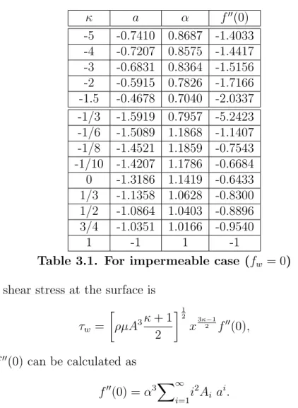
One of our main aim is to determine the value of f⁰⁰(0) which is the velocity gradient at the wall. It has an important physical meaning. It appears in drag force due to wall shear stress. For a solid object moving in a fluid, the drag force is a hydrodynamic force acting in the direction of the movement to oppose the motion. The drag force is proportional to the drag coefficient C_D,τ, the density and the velocity square. In general, C_D,τ is not an absolute constant. The drag coefficient is a non-dimensional quantity and it varies with the speed (or more generally with Reynolds number), the flow direction, the fluid density and fluid viscosity. The valuef⁰⁰(0) is used to call the skin friction parameter and it is involved in the drag coefficient

C_D,τ = (2)¹² Re⁻¹² f⁰⁰(0), and in the wall shear stress

τ_w =

ρµU_∞³ x

¹₂

f⁰⁰(0).

The velocity profiles measured at different distances x from the leading edge when represented in coordinate system u(x, y)/U∞ and y/x¹² collapse into one. So, the velocity profiles are similar to one another, the boundary layer is self-similar, i.e. they can be mapped onto one another by choosing suitable scaling factors.

Applying the similarity method, the two independent variables x and y are combined to form a new variable η in order to transform the partial differential equation (2.7) into an ordinary differential equation (2.10). In [212] Weyl has proved that there is a unique solution to the Blasius problem (2.10), (2.11).

(24)

2.1.3 T¨opfer transformation

In this section instead of the Blasius problem (2.10), (2.11) we consider the initial value problem

f⁰⁰⁰+ 1

2f f⁰⁰= 0,

f(0) = 0, f⁰(0) = 0, f⁰⁰(0) =γ.

The task is to determineγ such that the corresponding solution satisfies (2.10) and (2.11). T¨opfer [203] realized for the Blasius problem (2.10), (2.11) that the knowledge of γ is in fact unnecessary. The reason is that there is a second group invariance such that if g(η^∗) denotes the solution to the Blasius equation (2.10) with initial conditions g(0) = 0, g⁰(0) = 0, and for its second derivative g⁰⁰(0) = 1, then the solution f with initial conditions f(0) = 0, f⁰(0) = 0, f⁰⁰(0) =γ can be obtained as

(2.13) f(η) =γ^1/3g γ^1/3η

(see [203]). It therefore suffices to compute g(η^∗) and then rescale of g(η^∗) so that the rescaled function has the desired asymptotic behavior at large η, namely, f⁰(∞) = 1. The true value of the second derivative at the origin is then

γ = lim

η^∗→∞[g⁰(η^∗)]^−3/2.

With T¨opfer’s transformation, it is only necessary to solve the differential equation as an initial value problem.

This scaling invariance has both analytical and numerical interest. From numerical viewpoint this transformation allows us to find non-iterative numerical solutions by the related initial value problem. From a numerical point of view to calculate lim

η^∗→∞g⁰(η^∗) is not simple. The most widely used numerical technique to boundary value problems on infinite domains is to introduce a suitable truncated boundary η^∗_t instead of +∞. T¨opfer [203]

solved the initial value problem obtained for the Blasius equation (2.10) for a large but finite η^∗_j, ordered such that η_j^∗ < η_j+1^∗ . He computed the corresponding values of γ_j. If γ_j and γ_j+1 agree with a specified accuracy, then γ is approximated by the common value of γ_j and γ_j+1. T¨opfer kept repeating his calculations with a larger value of η^∗.

Weyl [212] noted that the Blasius problem ”was the first boundary-layer problem to be numerically integrated . . . [in] 1907.”

(25)

2.1.4 Power series solutions

The Blasius function is defined as the unique solution to the boundary value problem (2.10), (2.11). Blasius [30] derived power series expansion which begins

(2.14) f(η)≈ 1

2γη²− 1

240γ²η⁵+ 11

161280γ³η⁸− 5

4257792γ⁴η¹¹+. . . , whereγ =f⁰⁰(0) is the curvature of the function at the origin. A closed form for the coefficients is not known. However, the coefficients can be computed for

f(η) =η²

∞

X

k=0

−1 2

k

A_kγ^k+1 (3k+ 2)!η^3k, from the recurrence

A_k=

k−1

X

j=0

3k−1 3r

A_rAk−r−1, if k≥2,

withA₀ =A₁ = 1.Hereγmust be numerically given. Howarth [109] obtained a numerical result γ ≈ 0.332057. Recently, Abbasbandy [1] proposed an Adomians’s decomposition method to the Blasius’s problem and obtained γ = 0.333329 with a 0.383% relative error of the initial slope, and Tajvidi et al. [197] has used a modified rational Legendre method, to show that γ = 0.33209 with a 0.009% relative error. By the fourth-order Runge-Kutta method γ is determined γ ≈ 0.33205733621519630, where all the sixteen decimal places are believed correct [56]. A fully analytical solution (i.e. not relying on any approximation) of the Blasius problem has been found by Liao [128] using the homotopy analysis method. He’s homotopy perturbation method has been successfully applied in fluid mechanics (see e.g. [15], [150], [219], [220]).

It should be noted that Blasius’ series has only a finite radius of convergence:

(2.15) ρ= lim

k→∞

(3k)(3k+ 1)(3k+ 2)Ak−1

A_kγ

¹₃

= 5.688.

The limitation of a finite radius of convergence can be overcome by con- structing power series by Pad´e approximants or an Euler-accelerated series, which both apparently converge for all positive real x [55].

(26)

Although the Blasius problem is almost a century old, it is still a topic of active current research (see e.g. [1], [5], [6], [55], [69], [84], [102], [103], [128], [206]).

A brief history of the numerical determination ofγ:

• (1912)γ = 0.332, T¨opfer [203]

• (1938)γ = 0.332057, Howarth [109]

• (1941) Weyl [212]

• (1941) John von Neumann

• (1948) Ostrowski [163]

• (1956) Meksyn [151]

• (1998) Fazio [86]

• (1999) Liao [128]

• (2006)γ = 0.33209, Tajvidi et al. [197]

• (2007)γ = 0.333293, Abbasbandy [1]

• (2008)γ = 0.33205733621519630, Boyd [56]

• (2011) Peker, Karao˘glu, Oturanc [166]

2.2 Non-Newtonian fluid flow with constant main stream velocity

Fluids such as molten plastics, pulps, slurries and emulsions, which do not obey the Newtonian law of viscosity are increasingly produced in the indus- try. By analogy with the Blasius description [30] for Newtonian fluid flows, similarity solutions can be studied and investigated to the model arising for a laminar boundary layer with power-law viscosity. The first analysis of the boundary layer approximations to power-law pseudoplastic fluids was given by Schowalter [179] in 1960. The author derived the equations governing the similarity flow. The numerical solutions were presented of the laminar flow of non-Newtonian power-law model past a two-dimensional horizontal surface by Acrivos, Shah and Petersen [4]. When the geometry of the surface is simple the system of differential equations can be examined in details and can be obtained fundamental information about the behavior of non-Newtonian fluids in motion (e.g., to predict the drag). The existence of a unique solution was proved in [25]. We show that a T¨opfer-like transformation can be applied for the determination of the dimensionless wall gradient and we provide power series solution near the wall [38]. Moreover, we can give a method for the determination of the power series approximation similar to Blasius’s form (2.14) for n >0.

(27)

2.2.1 Boundary layer governing equations

We consider two-dimensional steady flow of a viscous fluid with constant velocityU∞. The problem is a model for the the laminar incompressible flow of a non-Newtonian power-law fluid past a flat surface. The surface is located at y= 0.

The analysis is restricted to the cases when the usual boundary layer approximations can be made, for large Reynolds numbers, defined for power- law fluids by

(2.16) Re = ρU_∞²⁻ⁿLⁿ

K .

This allows to simplify the basic equations of conservation of momentum and mass. The problem is deduced from the boundary layer approximation (1.1), (1.6), where the shear stress τyx is given by the power-law expression (1.11):

∂u

∂x +∂v

∂y = 0, (2.17)

ρ

u∂u

∂x +v∂u

∂y

= K ∂

∂y

∂u

∂y

n−1 ∂u

∂y

! . (2.18)

At the solid surface the usual impermeability and no-slip are applied and outside the viscous boundary layer the streamwise velocity component u should approach the exterior streaming speed U∞:

(2.19) u(x,0) = 0, v(x,0) = 0, lim

y→∞u(x, y) = U∞.

The boundary layer equations (2.17) and (2.18) are nonlinear and have boundary conditions at 0 and at +∞.

Introducing the stream function ψ defined in (2.6), the continuity equation (1.1) is automatically satisfied and (2.18) can be written as

(2.20) ∂ψ

∂y

∂²ψ

∂y∂x −∂ψ

∂x

∂²ψ

∂y² =µcn

∂

∂y

"

∂²ψ

∂y²

n−1 ∂²ψ

∂y²

#

, µcn =K/ρ.

Boundary conditions in (2.19) can be formulated as

(2.21) ∂ψ

∂y (x,0) = 0, ∂ψ

∂x (x,0) = 0, and

(2.22) lim

y→∞

∂ψ

∂y (x,0) = U_∞,

(28)

where the unknown function is the stream function ψ.

Let us define the stream functionψ and similarity variable η such as ψ =Ax^αf(η), η=Bx^βy,

where A, B, α and β are constants to be determined, and f(η) denotes the dimensionless stream function. Choosingβ =−αandAB=U∞, the boundary value problem (2.20)-(2.22) is transformed by means of dimensionless variables ([4], [25], [38],[179])

(2.23) ψ(x, y) =µ

1

cnn+1U

2n−1

∞n+1xⁿ⁺¹¹ f(η),

(2.24) η=µ⁻

1

cnn+1U

2−n

∞n+1

y xⁿ⁺¹¹ into the so-called generalized Blasius problem

(2.25)

|f⁰⁰|ⁿ⁻¹f⁰⁰⁰

+ 1

n+ 1f f⁰⁰ = 0, (2.26) f(0) = 0, f⁰(0) = 0, lim

η→∞f⁰(η) = 1,

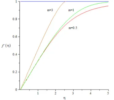
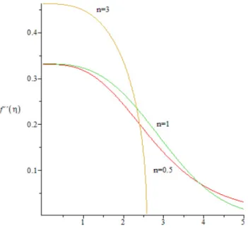
where the prime denotes the differentiation with respect to the similarity variable η and the non-dimensional velocity components are obtained by f as follows:

u(x, y) = U∞f⁰(η), v(x, y) = v^∗(x) [ηf⁰(η)−f(η)], with

v^∗(x) = U∞

n+ 1Re⁻

1

xn+1,

when for power-law non-Newtonian fluids the local Reynolds number Re_x is defined by

Re_x = ρU_∞²⁻ⁿxⁿ

K .

If n = 1, equation (2.25) is the same as the famous Blasius equation (2.10).

Equation (2.25) is nonlinear except in the case n= 2, when explicit solution exists. For detailed analysis we refer to the paper by Liao [129].

Since the boundary layer equations are valid when the Reynolds number is large, it is worth to examine under what conditions laminar boundary layer flows would be expected to occur. In [4] the following conclusions were

(29)

deduced:

(i.) IfU∞is sufficiently small and the inertia terms of the equations of motion may be neglected, all fluids approach Newtonian behavior.

(ii.) If n < 2, boundary layer type flow can be obtained when U_∞ is large and therefore the Reynolds number is sufficiently large.

(iii.) If n > 2, boundary layer type flow can be obtained for moderate values of U_∞ when the Reynolds number is large. If U_∞ is too large then Re will be small. So, if U∞ is sufficiently large the boundary layer flow is not an asymptotic state of laminar motion. If U∞ tends to zero then Re tends to ∞ and the characteristic velocity is small as the model (1.11) is valid when ∂u/∂y is relatively large. When U∞ and therefore ∂u/∂y is small non-Newtonian boundary layer flow do not occur. So, for n > 2, the laminar boundary layer flows are probably not of interest because their range of validity is rather limited.

For the numerical solution to (2.25), (2.26) we refer to the paper by Acrivos et al. [4] when the Polhausen-type momentum integral method was applied for the determination of the velocity distribution and the shear stress at the wall. It should be noted that when n ≥ 2 there is no solution f to (2.25), (2.26). Then, the boundary condition at infinity in (2.26) has to be changed

(2.27) f(0) = 0, f⁰(0) = 0, f⁰(η) = 1, for η≥η₀,

where η₀ = ∞ for n < 2 and η₀ is finite for n ≥ 2. The phenomenon of a finite η₀ has not appeared in the case of laminar Newtonian boundary layer fluid flows.

2.2.2 T¨opfer-like transformation

Here we want to provide a transformation similar to T¨opfer’s transformation for power-law type viscosity. We replace the condition at infinity by one at η = 0. Therefore, the generalized Blasius problem (2.25), (2.26) is converted into the initial value problem

(2.28)

|f⁰⁰|ⁿ⁻¹f⁰⁰0

+ 1

n+ 1f f⁰⁰= 0, (2.29) f(0) = 0, f⁰(0) = 0, f⁰⁰(0) =γ.

The solution can be obtained if onlyγ =f⁰⁰(0) were known such that the corresponding solution satisfies (2.25), (2.26).

(30)

We present a modified version of T¨opfer-method for non-Newtonian fluid flows [38]. In order to transform the boundary value problem (2.25), (2.26) into an initial value problem let us introduce the scaling transformation

(2.30) g =λ^κf, η^∗ =λη,

where κ and are real, non-zero parameters. Our aim is to determine κ and such that the boundary conditions are substituted by suitable initial conditions. After simple calculations we have

df

dη =λ^κ− dg

dη^∗, d²f

dη² =λ^κ−2 d²g

dη^∗2, d³f

dη^∗3 =λ^κ−3 d³g dη^∗3.

The governing differential equation is left invariant by the new variables g and η^∗

(2.31)

|g⁰⁰|ⁿ⁻¹g⁰⁰⁰

+ 1

n+ 1gg⁰⁰ = 0,

where the prime for g denotes the derivatives with respect toη^∗, when κ(2−n) = (1−2n).

The initial conditions in (2.29) correspond to

(2.32) g(0) = 0, g⁰(0) = 0,

moreover, with the choice of λ=γ, one gets

g⁰⁰(0) =γ^κ−2f⁰⁰(0) =γ^κ−2+1.

So, with κ= ¹⁻²ⁿ₃ and = ²⁻ⁿ₃ , i.e., g =γ¹⁻²ⁿ³ f, η^∗ =γ²⁻ⁿ³ η, we obtain

(2.33) g⁰⁰(0) = 1.

Then

f(η) = γ^(2n−1)/3g γ^(2−n)/3η ,

which is reduced to T¨opfer’s form (2.13) for Newtonian fluid (n= 1). Value γ will be determined by the boundary condition at +∞ in (2.29) such as

1 = lim

η→∞f⁰(η) = lim

η^∗→∞γ^κ−g⁰(η^∗) = lim

η^∗→∞γⁿ⁺¹³ g⁰(η^∗), that is

ηlim^∗→∞g⁰(η^∗)) =γ⁻ⁿ⁺¹³ ,

(31)

and hence

γ = lim

η^∗→∞[g⁰(η^∗)]⁻ⁿ⁺¹³ .

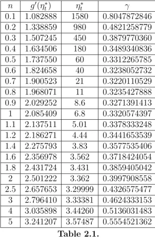
Table 2.1 shows numerical results forη^∗_t of the solutions to (2.31)-(2.33) for n-values between 0.1 and 5. Here we represent suitable truncated boundaries η_t^∗ instead of +∞.

The classical fourth-order Runge-Kutta method is applied and a local error of the order of 10⁻⁶ is maintained. Table 2.1 also contains the corresponding values, g⁰(η^∗_t), and the values of γ for n-values between 0.1 and 5 such thatγ = [f^∗0(η^∗_t)]^−3/(n+1) with the present numerical techniques. These values give approximations for the dimensionless wall gradient, with f⁰⁰(0) represented for n-values between 0.1 and 25 in Fig. 2.5.

n g⁰(η_t^∗) η_t^∗ γ 0.1 1.082888 1580 0.8047872846 0.2 1.338859 980 0.4821258779 0.3 1.507245 450 0.3879770360 0.4 1.634506 180 0.3489340836 0.5 1.737550 60 0.3312265785 0.6 1.824658 40 0.3238052732 0.7 1.900523 21 0.3220110529 0.8 1.968071 11 0.3235427888 0.9 2.029252 8.6 0.3271391413 1 2.085409 6.8 0.3320574397 1.1 2.137511 5.01 0.3378333248 1.2 2.186271 4.44 0.3441653539 1.4 2.275793 3.83 0.3577535406 1.6 2.356978 3.562 0.3718424054 1.8 2.431724 3.431 0.3859405042 2 2.501222 3.362 0.3997908558 2.5 2.657653 3.29999 0.4326575477 3 2.796410 3.33381 0.4624333153 4 3.035898 3.44260 0.5136031483 5 3.241207 3.57487 0.5554521362

Table 2.1.

Since the pioneering work by Acrivos et al. [4], different approaches have been investigated for γ in the case of non-Newtonian fluids. It has a physical meaning. It appears in drag force due to wall shear stress which is a fluid dynamic force. The skin friction parameter γ originates from the wall shear