Estimation of Recycling Capacity of Multi-storey Building Structures Using Artificial Neural Networks

(1)

Estimation of Recycling Capacity of Multi- storey Building Structures Using Artificial Neural Networks

Vladimir Mučenski

¹

, Milan Trivunić

¹

, Goran Ćirović

²

, Igor Peško

¹

, Jasmina Dražić

¹

1 University of Novi Sad, Faculty of Technical Sciences, Department of Civil Engineering and Geodesy, Trg Dositeja Obradovića 6, 21000 Novi Sad, Republic of Serbia, mucenskiv@uns.ac.rs, trule@uns.ac.rs, igorbp@uns.ac.rs,

dramina@uns.ac.rs

3 Belgrade University, College of Applied Studies in Civil Engineering and Geodesy, Department of Civil Engineering, Hajduk Stankova 2, 11000 Belgrade Republic of Serbia, cirovic@sezampro.rs

Abstract: In recent years, we are witnessing a greater tendency towards the use of existing construction waste, in order to reduce the amount of material being disposed of on the one hand, and to limit the exploitation of natural resources necessary for the production of construction materials on the other hand. This paper provides an outline of a process for predicting the recyclable amount of concrete and reinforcement built in structures of residential buildings based on artificial neural networks (ANN). The following analyses are included in the process: an analysis of the optimal network structure, analysis of the effect of training algorithms and a network sensitivity analysis. While analyzing these, networks with one and two hidden layers trained with 5 algorithms (Gradient descent with adaptive lr backpropagation, Levenberg-Marquardt backpropagation, quasi-Newton backpropagation, Bayesian regularization and Powell-Beale conjugate gradient backpropagation) for neural network training were observed. The research was carried out with the purpose of observing ANN that will quickly and with adequate precision provide information regarding the amounts of concrete and reinforcement that can be recycled.

Keywords: Recycling; concrete; reinforcement; prediction of the quantity; artificial neural network; training algorithm; sensitivity analysis

1 Introduction

An increase in the use of recycled materials has become an imperative in the process of environmental protection. The need to create a sustainable production system within which the exploitation of natural resources and the amounts of waste materials will be reduced to a minimum has been present in construction industry for years.

(2)

The issue of estimating recycling capacities of building constructions is of crucial importance for establishing financially justifiable recycling processes and for the re-use of construction materials. In the Republic of Serbia, 22,272,500 m² of flats are older than 65 years, and 74,053,973 m² are older than 40 years, which presents a significant recycling potential when it comes to construction materials. In order to estimate the amount of concrete and reinforcement to be recycled in relation to the characteristics of a building as accurately as possible, it is necessary to analyze several parameters which describe the building, with parameters of both quantitative and qualitative nature. In such cases, statistical methods do not provide sufficiently accurate results.

With the development of software for solving mathematical problems, but also with the development of a totally new concept of programming and calculation within the same, known as “soft computing”, the opportunity became available for using particular mathematical concepts, the realization of which, up to that point, had not been possible for very complex problems.

One of these concepts is that of artificial neural networks, which attempts to simulate the working of the human brain in order to solve particular mathematical problems. As the amount of research using neural networks has increased, so has the number of attempts to apply them in the construction industry, on the basis of which it can be confirmed that their use is more than justified.

The aim of this paper is to develop such a model for the estimation of the amount of recyclable concrete and reinforcement, one which does not require the use of project documentation or data which cannot be collected by visual examination of a building. The reason for this lies in a lack of projects for a large number of building constructions within the archive.

For this reason, research was carried out into the use of artificial neural networks for predicting the amount of recyclable concrete and reinforcement built in the skeletal structure of residential buildings. The prediction of the amount of materials was done on the basis of a database formed for the purposes of this research; the database included 9 parameters: the (complexity of the building, the total gross area of the building, the average gross floor area, the height of the building, the number of stiffening walls, the longitudinal and transverse raster of the construction, the type of floor structure and the type of floor support structure.

All are available or can be easily defined based on project documentation. The output values of the database are the amounts of concrete and reinforcement.

In this paper, a brief overview of the concept of artificial neural networks is given, as well as an overview of the current situation regarding their application in solving a given problem. Additionally, a detailed methodology is given for the implementation of research into predicting the amount of materials required, which includes: the process of forming a database, the process of finding the optimal network architecture, the process of finding an optimal training algorithm and the process of sensitivity analysis of the network on the input data.

(3)

2 The Fundamentals of Artificial Neural Networks

The basic logical scheme for the imitation of the biological nervous system was formed by McCulloch and Pitts, who defined the mathematical principles which enabled the formation of artificial neural networks [1]. The principle of artificial neural networks is based on the attempt to imitate the biological nervous system in which artificial neural networks support the recognition of particular regularities and their memorization. In addition, gradual learning is possible during their application, i.e. adapting already established rules within the given network.

Because of their flexibility in finding dependence, artificial neural networks are suitable for analyzing problems for which there is no clear describable mathematical dependence. There are many definitions of artificial neural networks. Hajkin defines them as huge distributed parallel processors [2]; Zurada regards them as physical cellular systems which can learn, memorize and use experimental knowledge [3]; and Nigrin defines them as systems which consist of a large number of simple elements for processing information [4].

If one wants to form a mathematical model of a biological neuron, particular respect must be paid to its structure. Dendrites, the body of the neuron and the axon must be formed. Figure 1 shows the McCulloch-Pitts general model of a mathematical neuron, the so-called M-P neuron, which has been used for the purpose of this research [5]. The weighted input section of the neuron represents the dendrites. In the body of the neuron, the summing of the signal occurs, on the basis of which the neuron is activated or not. If activation occurs, a signal is sent via the output (axon) to the neurons to which it is connected.

a(·) θi

Σ x1

x2

xm

wi1

wi2

wim

yi inputs

weights

output Transfer function

Figure 1

The McCulloch-Pitts model of an artificial neuron

Neurons are interconnected, forming a network where they can be arranged either within a single or several layers. The number of neurons can vary from one layer to another. The acquired network structure has a great impact on the speed and quality of neural network training. The process of finding the optimal structure is iterative.

In addition to defining the network structure and the number of neurons, it is necessary to choose the manner of network training. Network training is based upon finding regularities by the network based on a sufficient amount of data given in order to determine interdependence. The result of a network training

(4)

process is the values of weight coefficients which describe links between neurons, as was explained earlier, and/or the change in the neural network structure.

Considering all of this, we can distinguish between two basic types of networks [6]:

 fixed networks, in which the weights cannot be changed, i.e. dW/dt=0. In such networks, the weights are fixed a priori according to the problem to solved and

 adaptive networks, which are able to change their weights, i.e. dW/dt≠0.

The weights change according to adopted learning rules, such as the Hebbian learning rule, the correlation learning rule, the instar learning rule, winner takes all, the outstar learning rule, the Widrow-Hoff LMS learning rule, linear regresion and the delta learning rule.

The neural network learning process is carried out by using learning algorithms.

All learning algorithms used for adaptive neural networks can be classified into two major categories:

 supervised learning, which incorporates an external teacher, so that each output unit is told what its desired response to input signals ought to be, and

 unsupervised learning, which uses no external teacher and is based upon only local information. It is also referred to as self-organisation, in the sense that it self-organises data presented to the network and detects their emergent collective properties.

Combining and summing of the input data and the weight coefficient occur in the input of the neuron. Output of the neuron is defined by the transfer function “a”

which activates or prevents activation of the observed neuron depending on the output value of the function. This function typically falls into one of three categories: linear (or ramp), threshold or sigmoid.

For our research purposes, a supervised adaptive network and two types of transfer functions were used:

 hyperbolic tangent sigmoid function

f 1 e λ 1 f 2

a -

+ - )=

( (1)

 and linear function.

f f

a( )= (2)

(5)

3 Review of Relevant Literature

Research up to now has been based on the use of both statistical models and ANN when establishing dependence between parameters which describe a building construction and the building costs. Kim et al. [7] compared the efficiency of regression analysis and ANN when faced with the problem of predicting building costs, and concluded that ANNs offer a more precise estimate of the required data.

Wang and Gibson [8] carried out similar research by comparing the effectiveness of applying neural networks with regression analysis when predicting the success of a construction project in which one of the parameters of success was the project budget. Gunaydin and Dogan [9] analyzed the application of ANN in estimating the cost of building an RC construction in which costs were defined per m² of the area of the building. The analysis was conducted on the basis of 30 projects completed in Turkey, and the average error was 7%.

In addition, a large number of analyses were carried out using hybrid ANN models and fuzzy logic and/or genetic algorithms. Yu and Skibniewski [10]

formed a hybrid neuro-fuzzy model for finding the optimal technology for constructing buildings based on technologicity.Kim et al. [11] analyzed the use of ANN with optimization of the same using genetic algorithms during the estimation of construction costs. For this they used a database containing information on 530 residential buildings. The result of using a hybrid model was that 80% of the data for validating the network was found in a error interval of up to 5%. Cheng et al. [12] analyzed the application of fuzzy ANN for predicting conceptual construction costs, whereby they evaluated the significance of 47 building parameters. The research resulted in an average error estimate of 5.9%.

On the other hand, Cheng et al. [13] formed the Evolutionary Web-based Conceptual Cost Estimator (EWCCE), a hybrid model including WWW, genetic algorithms, neural networks and fuzzy logic with the purpose of estimating construction costs in the early stages of a project. The accuracy of the model was greater than 75%. It should be noted that research dealing with the prediction of the quantities of materials that could be recycled is rare.

4 Data Collection and Database Creation

The quality of a neural network depends on the amount and quality of the data on the basis of which the neural network is trained. For this reason, for the purposes of this research, a database was established containing information from major residential building construction projects in Novi Sad, Republic of Serbia. The data was randomly divided into two groups, namely: a data set for training the neural network (95 projects) and a data set for evaluating the quality of the analyzed network (15 projects). The parameters chosen for describing the characteristics of the structure are shown in Table 1 and include the geometric and structural characteristics of the building.

(6)

Table 1

Contains the result of comparing in pairs with the final result

Type

Building paramet er

Definition Paramet

er type Interval or parameter definition

Input data

x1

Complexity of

the building Discrete Simple (1), medium (2), complex (3), very complex (4)

x2 Total gross area Numeric 1000m² - 8000m² x₃ Average gross

floor area Numeric 200m² - 2000m² x4 Building height Numeric 13m – 27m x₅ Number of

stiffening walls Numeric 0 – 13 x6

Longitudinal

raster Discrete 1.00m-1.99m (1); 2.00m-2.99m (2); 3.00m-3.99m (3); 4.00m- 4.99m (4); 5.00m-5.99m (5);

6.00m-6.99m (6); 7.00m-7.99m (7) x7

Transverse

raster Discrete

x₈ Type of floor

structure Discrete

Full RC slab (1), Semi-

prefabricated ceiling type “FERT'' (2)

x9

Type of supporting floor structure

Discrete Direct support(1), girder support (2)

Outpu t data

y₁ Quantity of

concrete Numeric 420m³ - 4500 m³ y2

Quantity of

reinforcement Numeric 28500kg – 310000kg

It should be noted that all the analyzed buildings have base slab support. In addition to the above, the database also includes buildings with one or without any dilation since this is the case in over 95% of residential buildings in the analyzed area.

The complexity of the building was adopted because of attempts to define the influence of the building's characteristics from the aspect of the complexity of the construction and the shape of the building on the output values. Included in simple buildings are buildings with a rectangular base and are without any changes in the construction of the floor. Medium complex buildings are characterized by particular changes in the construction of the floor or an approximately rectangular base with fewer deviations (L base). In the category of complex buildings are those with an indented base (П base, H base and so on), while very complex buildings are characterized by an indented base and/or atypical changes in the floor construction such as a reduction in the floor area with a growth in its height and an atypical shape of the skeletal construction.

(7)

The total area of the building is a parameter which is expected to have a great influence on the quantity of materials. Here, the gross area was taken into account to make prediction easier.

Including the floor area is an additional attempt to establish a correlation between the shape, i.e. the footprint of the building and the output values. In doing this, the gross floor area was also adopted.

The definition adopted for the height of the building was the distance from the ground surface to the highest point of the building.

Given that the seismic resistance of the building (and with that the amount of concrete and reinforcement) above all depends on the number and the distribution of stiffening walls, the influence of the same on the output values was adopted.

The size of the longitudinal and transverse raster of structure has a direct influence on the span of the girders and the ceiling. The interval range and adopted parameters are shown in Table 1.

During data collection, two types of floor structure and two types of supporting floor structure were dominant within the project, as shown in Table 1. Table 2 shows the segments of the data base on the basis of which training and validation of the ANN were carried out.

Table 2

Segments of the input and output data sets for the training and validation of neural networks

Input data Output data

x₁ x₂ x₃ x₄ x₅ x₆ x₇ x₈ x₉ y₁ y₂

3 2000 250 23 5 5 3 1 1 800 86000

2 4700 790 17 6 4 5 1 1 1870 148000

2 4350 830 18 8 5 5 1 1 2100 152000

2 2250 340 22 5 3 3 2 2 1050 66500

When considering the limitations of the database, it should be noted that it includes only buildings which have a concrete skeletal system. In addition to the above, the limits of the established base represent the minimum and maximum data values on the basis of which the ANN is trained. That is, when carrying out an estimate of the amount of materials for a new building, the parameter values must be found within the interval of the data collected so that it is possible to analyze only the options with the analyzed types of base structure, floor structure and the support of the same.

Taking into account that there is a clear distinction in the order of magnitude of the data from 0 to 10⁵ (see Table 2), it is necessary to prepare the data in order for it all to be analyzed equally, i.e. it is necessary to carry out normalization of the data. Normalization of the data leads to an increase in the performance of the trained ANN [9]. Based on the above, normalization of the whole database was carried out, i.e. the input and output data both in the training set and in the testing

(8)

set for the ANN. Normalization of the data was performed using “Z-Score” [14]

transformation in the distribution where the mean is (μ) 0, and the standard deviation (σ) 1 using the following expression:

σi μi Xij ij

-

=

S (3)

where: S_ij – is the normalized data value X_ij – is the actual data value

μi – is the mean distribution (data set for training)

σi – is the standard deviation of the distribution (data set for training) i – is the input (i = i₁, i₂,..., i₉) or output (i = o₁, o₂) data

j – is the number of combinations (j = 1, 2,…, n); n – is the number of data sets.

Of course, given that training of the ANN is carried out based on normalized data, the output from the ANN is also normalized. It is necessary to transform the output in order to obtain real values comparable with the expected values from the data sets for testing the ANN on the basis of which error is determined [14].

Transformation is performed using the following expression:

i ij i ij NN

real S σ μ

X = • + (4)

where: S^NN_ij – is the normalized data value obtained as output from the ANN X^real_ij – is the real data value obtained on the basis of S^NN_ij

μi – is the mean distribution (data set for training)

σi – is the standard deviation of the distribution (data set for training) i – is the output data (i = o₁, o₂)

j – is the number of combinations (j = 1, 2,..., m); m – is the number of data sets for testing.

5 ANN Analyses for Predicting the Quantity of Recycling Material

In this part of the study we present a detailed overview of the process of using neural networks for predicting the quantity of recyclable concrete and reinforcement. The process is presented for finding the optimal network architecture and optimal algorithm for training the network, along with a sensitivity analysis of the network on the input data used for training the network.

(9)

5.1 Modelling the ANN

The type and the structure of a neural network have a significant effect on the quality and efficiency of the network. ANNs consist of neurons in layers, the number of which depends primarily on the problem being solved by the network.

Based on research, a conclusion was drawn that networks with a small number of neurons (in relation to the optimal number of neurons for the given problem) offer solutions with a rough approximation, i.e. with large deviations. On the other hand, too large a number of neurons gives too precise an approximation taking into account the small deviation when searching for dependence [15]. In addition to the number of neurons, the manner of grouping them in so-called layers of neurons is also significant. Therefore, we distinguish between single-layered and multi-layered networks.

In the phase of defining the ANN model, the required amount of input and output data is defined first. The number of input parameters determines the spatial dimensions of the network and the number of output parameters determines the number of solution surfaces generated by the network [16, 17]. The amount of input data is defined by the formation of a database based on the analysis carried out as to the significance of individual data, while the amount of output data is defined by the amount of information required as the end result of the application of a neural network.

An important characteristic of neural networks, in addition to the number of neurons and layers, is the method of data processing, i.e. the transfer flow of information between neurons. Therefore, we distinguish between forward oriented networks (the transfer of information takes place in one direction, forwards) and networks oriented backwards (the transfer of information takes place in both directions, forwards and backwards). In these, the networks mostly used are those with back propagation of errors where the signal is transmitted forwards, while the error is transmitted backwards in order to minimize it, and the whole process is repeated until the error reaches its minimum [9, 11, 18-21]. In view of the above, an algorithm with error backpropagation was used for the purposes of this research.

The process of finding the optimal structure of neural networks in its essence is examining different structures on the basis of the same set of data where the investigation involves varying the number of layers and the number of neurons in the network. The process of determining the quality of the network structure in relation to the given problem is based on determining the size of the error which is obtained as an output result after the network training process. Neural networks were applied to the given problem using the Matlab R2007b software package, on which the analysis of the structure, the training of the network and the simulation of the working of the same were carried out. The network type was not varied, since it was shown that networks with error backpropagation were optimal for the problem of prediction [7-9, 11, 19].

(10)

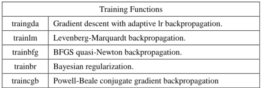
In the research presented in this paper, different training functions were used (see Table 3) in order to see their effect on the ANN modelling.

Table 3 Used training functions

Training Functions

traingda Gradient descent with adaptive lr backpropagation.

trainlm Levenberg-Marquardt backpropagation.

trainbfg BFGS quasi-Newton backpropagation.

trainbr Bayesian regularization.

traincgb Powell-Beale conjugate gradient backpropagation

In addition to defining the network type, it is necessary to define the number of layers and the number of neurons along with the transfer function in the neurons, which define the method of data transmission between the same.

For the observed network, the hyperbolic tangent sigmoid transfer function was used in the hidden layers except for in the output layers of the network for which a linear transfer function was used.

The research was carried out on two types of neural networks. The first type included networks with one hidden layer, whereas the second consisted of networks with two hidden layers. For each type, 4 versions of a neural network with different number and ordering of neurons in layers were analyzed (see Table 4). Previous research has shown that networks more complex than networks presented in table 4 are unstable in prediction and less accurate [22]. In Figure 2 some of the analyzed networks are shown. Figure 2a shows the network 2-2, which contains one hidden layer with two neurons, and the output layer, which also contains two neurons considering 2 outputs, whereas Figure 2c presents a network with three neurons in its hidden layer. Figure 2c shows the network 2-2-2 containing two hidden layers each with two neurons, as well as the output layer containing two neurons considering 2 outputs.

i5

i₄ i3

i2

i₁

i9

i8

i7

i6

o1

o2

b)

i5

i4

i3

i2

i₁

i9

i8

i₇ i6

o1

o₂ a)

i5

i₄ i3

i2

i1

i9

i8

i7

i6

o1

o2

c)

Figure 2

Models of ANN used with 9 inputs; (a) network 2-2, (b) network 3-2, (c) network 2-2-2

(11)

Testing the ANN, i.e. the evaluation of its performance, can be done on the basis of different criteria. In this research the performance of the ANN was evaluated on the basis of MAPE (mean absolute percent error) using the following expression:

%

•100 n

1

i= actuali

di -predicte actuali

n

MAPE=1

∑

⁽⁵⁾

where n – is the number of data sets for testing.

Testing was conducted on 15 sets of input and output data which were not taken into account when the network was being trained. In addition to testing all the neural networks on the basis of MAPE, their stability was also tested. The control of the network stability was realized by comparing MAPE output results obtained through testing networks for 4 consecutive testing iterations; i.e. for each version of the network, 4 tests were carried out. If MAPE differs from the iterations of prediction the network is considered unstable, i.e. it will not always carry out a prediction with the same accuracy. Apart from MAPE, control of stability of network sensitivity on input parameters was also carried out, defining the impact of input parameters on the result. If the significance of input data varied within the four analyzed iterations, the network was considered to be unstable; i.e. the network was only considered to be stable provided that it gave the same results of MAPE and the significance of input parameters for all four testing iterations.

Table 4

MAPE and stability of analyzed networks with nine input parameters

Training

functions Output

one hidden layer two hidden layers

number of neurons in hidden layer - number of neurons in output layer

number of neurons in hidden layer 1 - number of neurons in hidden layer 2 - number of neurons in output layer

2-2 3-2 4-2 5-2 2-1-2 2-2-2 3-2-2 2-3-2

traingda

concrete

unstable unstable unstable unstable unstable unstable unstable unstable reinforcement

trainlm

concrete

trainbfg

concrete

trainbr

concrete 11.55% 14.22%

unstable unstable unstable unstable unstable unstable reinforcement 8.93% 13.73%

average 10.24% 13.98%

traincgb

concrete

(12)

As can be seen in Table 4, stable networks were only present in the case when there was one hidden layer of neurons that contains two or three neurons, where the network was trained by trainbr function (Bayesian regularization). At the same time, the network with 2 neurons in the hidden layer provides higher accuracy of prediction compared with the network with 3 neurons in the hidden layer. For the network trainbr 2-2, MAPE_average=10,24% , whereas for the network trainbr 3-2, MAPE_average=13,98%. Figures 3 and 4 show the values of PE (percentage error, equation 6) for the two chosen networks (trainbr 2-2 and trainbr 3-2).

%

•100 actuali

-actuali predictedi

PE= (6)

Figure 3

The PE graphic of each individual piece of data for testing trainbr 2-2 (network with nine inputs)

Figure 4

The PE graphic of each individual piece of data for testing trainbr 3-2 (network with nine inputs) Observing Figures 3 and 4, a conclusion can be drawn that trainbr 2-2 network provides smaller errors of the output data, where the maximum error in predicting the amount of concrete is 27.36%, and the maximum error in the prediction of the amount of reinforcement is 27.49%.

-18.32 -1.43

2.60 7.03 8.64

-20.04 9.95

25.68 20.65

-0.46 -5.23

-27.36 -0.88

-19.66 1.90

-3.42 -5.26 -0.61 -4.33

-12.51 27.49

8.39 20.91

-2.34 -4.28

1.76

-21.52 14.04

5.14

PE (estimation of recyclable amount of concrete) PE (estimation of recycaible amount of reinforcement)

-15.98 5.49

1.54 7.25

14.60

-15.41 19.29

33.30 35.37

8.50

-3.17 12.26

-23.66 1.90

-15.66 4.61 3.21

-6.17

0.71 2.18

-6.78 37.02

13.44 29.48

16.03

-8.59 27.43

-19.00 18.94

12.39

PE (estimation of recyclable amount of concrete) PE (estimation of recyclable amount of reinforcement)

(13)

In order to realize the significance of input parameters on the output results, the sensitivity analyses of the observed networks was carried out. Sensitivity analysis provides vital insights into the usefulness of individual input variables. Through sensitivity analysis, variables that do not have significant effect can be taken out of the neural network model and key variables can be identified [20]. Sensitivity analysis results are shown within Figure 5.

Figure 5

Sensitivity analysis (network with nine inputs)

Based on Figure 5, it is possible to conclude that in the case of the observed networks, the most significant parameters are total gross area of the building (37.55%), transverse raster (15.80%), longitudinal raster (12.72%) and gross floor area (12.06%). These parameters are adopted for the further analysis since their significance exceeds 10%. Training and testing of the ANN were carried out again, but instead of using nine inputs, only the four were used

An analysis was carried out identical to the one for the previous input data. The analysis results are presented in Table 5. Fig. 6 shows a PE graph for the data set for testing the ANN (network with four inputs) obtained on the basis of PE (percentage error).

Table 5

MAPE of analyzed networks with four input parameters

Training

functions Output

One hidden layer

Number of neurons in hidden layer - number of neurons in output layer

2-2 3-2

trainbr

concrete 9.32% 9.47%

reinforcement 8.87% 10.82%

average 9.10% 10.15%

2.86%

37.55%

12.06%

7.29% 5.96%

12.72%

15.80%

4.04%

1.73%

Complexity Total gross area of the building

Gross floor area

Building height

Number of stiffening walls

Longitudinal raster

Transverse raster

Type of floor structure

Type of supporting floor structure

(14)

If tables 4 and 5 are compared, it is possible to draw the conclusion that the network trainbr 2-2 trained with 4 input parameters provides the most accurate prediction of the recyclable amount of concrete and reinforcement (MAPE_average=9.10%). At the same time, the network trainbr 2-2 provides the most accurate prediction of the amount of concrete (MAPE_concrete=9.32%), as well as the most accurate prediction of the amount of reinforcement (MAPEreinforcement=8.87%).

In Fig. 6 and Fig. 7 is a PE graph for the data set for testing the ANN (network with four inputs) obtained on the basis of PE (percentage error).

Figure 6

The Graphic PE of each individual piece of data for testing trainbr 2-2 (network with four inputs)

Figure 7

The Graphic PE of each individual piece of data for testing trainbr 3-2 (network with four inputs) If Figures 3 and 6 are compared, it is possible to conclude that after removing 5 input parameters for the network trainbr 2-2, the maximum error of prediction of the amount of reinforcement was reduced from 27.49% to 22.66%, as well as from 27.36% to 21.61% regarding the amount of concrete. Considerable progress was made for the network trainbr 3-2, resulting in a significant reduction in the

-15.75

3.39 5.31 5.96 2.99

-14.60 10.33

19.62 11.86

-8.23

0.42 1.86

-22.66 0.89

-15.95 1.06 2.68

-7.82 -2.94

-9.45 -10.15 21.61

9.66 8.42

-6.59 -5.97 9.47

-17.78 12.31

7.20

PE (estimation of recyclable amount of concrete) PE (estimation of recycaible amount of reinforcement)

-18.83

2.86 5.73 6.99

-0.75

-15.24 4.41

22.71

5.94

-13.74

0.68 1.07

-26.30 0.88

-15.97 -1.73

1.12

-9.22 -2.18

-16.39

-10.62 22.25

10.62 12.01

-11.20 -5.24

14.14

-24.63 13.83

7.10

PE (estimation of recyclable amount of concrete) PE (estimation of recyclable amount of reinforcement)

(15)

maximum error for the prediction of the amounts of both concrete and reinforcement. Maximum prediction error for the amount of concrete was reduced from 34.37% to 26.30%, whereas the maximum prediction error for the amount of reinforcement was reduced from 37.02% to 24.63%. Figure 8 shows the significance of input parameters for networks with 4 input parameters.

Figure 8

Sensitivity analysis (network with four inputs)

As can be seen in Figure 8, there was an increase in the significance of total gross area of the building and average gross floor area parameters, setting the balance between the significance of parameters relating to skeletal construction raster (longitudinal raster and transverse raster).

6 Discussion of the Results

During research into the applicability of ANN to the problem of predicting the quantities of concrete and reinforcement that can be recycled, a database of 110 residential building projects was created with 9 input parameters and 2 output parameters. The adopted input parameters are the following: complexity of the building, total gross area of the building, average gross floor area, building height, number of stiffening walls, longitudinal raster, transverse raster, type of floor structure, type of supporting floor structure. Before neural network training, preparation of data through “Z-Score” normalization was carried out.

Within the analysis, the networks with error backpropagation algorithms were observed, containing at the same time one hidden layer with 2 to 5 neurons as well as two hidden layers with 1 to 3 neurons. In network training, 5 training functions were used: traingda (Gradient descent with adaptive lr backpropagation), trainlm (Levenberg-Marquardt backpropagation), trainbfg (BFGS quasi-Newton backpropagation), trainbr (Bayesian regularization) and traincgb (Powell-Beale conjugate gradient backpropagation). As the first criterion for network validity, its

54.97%

16.12% 14.83% 14.08%

Total gross area of the building

Gross floor area Longitudinal raster Transverse raster

(16)

stability was adopted, where the observed results were obtained through 4 consecutive iterations for the same values of data. In doing so, stability of the obtained values of MAPE was observed, as well as the stability of sensitivity analysis on the input parameters. The network was regarded as stable only if it provided the same results of MAPE and input data significance for all 4 testing iterations. After analyzing 40 networks in 160 training and testing processes, a conclusion was reached that only networks with one hidden layer containing 2 or 3 neurons and trained with the trainbr function (Bayesian regularization) proved to be sable. The network trainbr 2-2 containing 2 neurons in its hidden layer and two in its output layer has an average error of prediction of the amount of concrete and reinforcement of 10.24%, whereas the network trainbr 3-2 containing 2 neurons in its hidden layer and two in its output layer displays an average error of 13.98%.

For the network trainbr 2-2, the individual error never exceeded the value of 27.49%, while in the case of trainbr 3-2 network the individual error never exceeded the value of 37.02%.

When analyzing the stability of the observed networks on the input parameters, a conclusion was drawn that four parameters have the strongest impact on the output results: total gross area of the building, average gross floor area, longitudinal raster and transverse raster. For this reason, the training process of the two observed networks was repeated with these 4 input parameters. By doing so, the average error of the output results for the network trainbr 2-2 was reduced from 10.24% to 9.10%, whereas for the network trainbr 3-2 the average error was reduced from 13.985 to 10.15%. In addition to reducing the average error, the maximum value of individual errors was also reduced. For the network trainbr 2- 2, the individual error did not exceed the value of 22.66%, whereas in the case of trainbr 3-2 network, the individual error did not exceed the value of 26.30%.

Based on all of the above, it can be concluded that for the observed problem, it is justified to train the network based on the 4 defined parameters. At the same time, the obtained results indicate that when collecting the data with the aim of data base expansion, particular attention should be paid to these input data.

Conclusions and Future Research

In this study is a presentation of the analysis and formation of networks for the purpose of predicting the amounts of recyclable concrete and reinforcement based on a database formed for the purposes of this research which contains data from 110 major residential building projects. It was concluded that for the given database, the best results are offered by a network with error backpropagation, and with one hidden layer of 2 neurons. When analyzing the results, a conclusion was reached that a network provides higher accuracy when it is trained with the 4 most significant parameters out of 9 which are defined within the base. The value of the average error of predicted amounts of concrete and reinforcement, compared with actual values, amounts to 9.10%.

(17)

Future research should be based on an expansion of the data base to other types of building constructions, as well as on other types of materials, such as brick, wood, ceramics, etc. In this way, a larger number of constructions suitable for recycling could be comprised, where it would be possible to determine a more comprehensive recycling capacity of a building construction, due to being able to predict the amounts of all the recyclable materials.

Acknowledgement

The work reported in this paper is a part of the investigation within the research project TR 36017 "Utilization of by-products and recycled waste materials in concrete composites in the scope of sustainable construction development in Serbia: investigation and environmental assessment of possible applications", supported by the Ministry for Science and Technology, Republic of Serbia. This support is gratefully acknowledged.

References

[1] W. McCulloch, W. Pitts, A Logical Calculus of the Ideas Immanent in Nervous Activity, Bulletin of Mathematical Biophysics, Vol. 5 (1943) 115- 133 http://www.cse.chalmers.se/~coquand/AUTOMATA/mcp.pdf (last visited on Oct. 17. 2011)

[2] S. Haykin, Neural Networks, Prentice Hall, New Jersy, 2005

[3] J. M. Zurada, Introduction to Neural Systems, West Publishing Company, St. Paul, 1992

[4] A. Nigrin, Neural Networks for Pattern Recognition, Cambridge MA: The MIT Press, 1993

[5] K. Kawaguchi, The McCulloch-Pitts Model of Neuron, http://wwwold.ece.utep.edu/research/webfuzzy/docs/kk-thesis/kk-thesis- html/node12.html (last visited on Feb. 15, 2011)

[6] http://www.doc.ic.ac.uk/~nd/surprise_96/journal/vol4/cs11/report.html (last visited on Feb. 01. 2013)

[7] G. H. Kim, S. H. An, K. I. Kang, Comparison of Construction Cost Estimating Models Based on Regression Analysis, Neural Networks, and Case-based Reasoning, Building and Environment, 39 (2004) 1235-1242 [8] Y. R. Wang, E. Gibson Jr., A Study of Preproject Planning and Project

Success Using ANNs and Regression Models, Automation in Construction 19 (2010) 341-346

[9] H. M. Gunaydın, S. Z. Dogan, A Neural Network Approach for Early Cost Estimation of Structural Systems of Buildings, International Journal of Project Management 22 (2004) 595-602

(18)

[10] W. Yu, M. J. Skibniewski, A Neuro-Fuzzy Computational Approach to Constructability Knowledge Acquisition for Construction Technology Evaluation, Automation in Construction 8 (1999) 539-552

[11] G. H. Kim, J. E. Yoon, S. H. An, H. H. Cho, K. I. Kang, Neural Network Model Incorporating a Genetic Algorithm in Estimating Construction Costs, Building and Environment 39 (2004) 1333-1340

[12] M. Z. Cheng, H. C. Tsai, E. Sudjono, Conceptual Cost Estimates Using Evolutionary Fuzzy Hybrid Neural Network for Projects in Construction Industry, Expert Systems with Applications 37 (2010) 4224-4231

[13] M. Y. Cheng, H. C. Tsai, W. S. Hsieh, Web-based Conceptual Cost Estimates for Construction Projects Using Evolutionary Fuzzy Neural Inference Model, Automation in Construction 18 (2009) 164-172

[14] J. S. Wu, J. Han, S. Annambhotla, S. Bryant, Artificial Neural Networks for Forecasting Watershed Runoff and Stream Flows. ASCE, Journal of Hydrologic Engineering, may/june (2005) 216-222

[15] H. Adeli, M. Wu, Regularization Neural Network for Construction Cost Estimation, Journal of Construction Engineering and Management, January/February (1998) 18-24

[16] I. Flood, N. Kartam, Neural Network in Civil Engineering I. ASCE, Journal of Computing in Civil Engineering, 8(2) (1994) 131-148

[17] I. Flood I, N. Kartam, Neural Network in Civil Engineering II. ASCE, Journal of Computing in Civil Engineering, 8(2) (1994) 149-162

[18] R. Rohas, Neural Networks, A Systematic Introduction, Springer-Verlag, Berlin, 1996, pp. 151-184

[19] S. Bhokha, S. Ogunlana, Application of Artificial Neural Network to Forecast Construction Duration of Buildings at the Predesign Stage Engineering, Construction and Architectural Management 6/2 (1999) 133- 144

[20] O. Tatari, M. Kucukvar, Cost Premium Prediction of Certified Green Buildings: A Neural Network Approach, Building and Environment 46 (2011) 1081-1086

[21] S. Rebano-Edwards, Modelling Perceptions of Building Quality—A Neural Network Approach, Building and Environment 42 (2007) 2762–2777 [22] V. Mučenski, I. Peško, M. Trivunić, J. Dražić, G., Ćirović, Optimization for

Estimating the Amount of Concrete and Reinforcement Required for Multi- storey Buildings, Building Materials and Structures 55(2) (2012) 27-46