Multidecadal trend analysis of in situ aerosol radiative properties around the world

(1)

https://doi.org/10.5194/acp-20-8867-2020

Multidecadal trend analysis of in situ aerosol radiative properties around the world

Martine Collaud Coen¹, Elisabeth Andrews^2,3, Andrés Alastuey⁴, Todor Petkov Arsov⁵, John Backman⁶, Benjamin T. Brem⁷, Nicolas Bukowiecki⁸, Cédric Couret⁹, Konstantinos Eleftheriadis¹⁰, Harald Flentje¹¹,

Markus Fiebig¹², Martin Gysel-Beer⁷, Jenny L. Hand¹³, András Hoffer¹⁴, Rakesh Hooda^6,15, Christoph Hueglin¹⁶, Warren Joubert¹⁷, Melita Keywood¹⁸, Jeong Eun Kim¹⁹, Sang-Woo Kim²⁰, Casper Labuschagne¹⁷, Neng-Huei Lin²¹, Yong Lin¹², Cathrine Lund Myhre¹², Krista Luoma²², Hassan Lyamani^23,24, Angela Marinoni²⁵,

Olga L. Mayol-Bracero²⁶, Nikos Mihalopoulos²⁷, Marco Pandolfi⁴, Natalia Prats²⁸, Anthony J. Prenni²⁹,

Jean-Philippe Putaud³⁰, Ludwig Ries⁹, Fabienne Reisen¹⁸, Karine Sellegri³¹, Sangeeta Sharma³², Patrick Sheridan³, James Patrick Sherman³³, Junying Sun³⁴, Gloria Titos^23,24, Elvis Torres²⁶, Thomas Tuch³⁵, Rolf Weller³⁶,

Alfred Wiedensohler³⁵, Paul Zieger^37,38, and Paolo Laj^39,40,41

1Federal Office of Meteorology and Climatology, MeteoSwiss, Payerne, Switzerland

2Cooperative Institute for Research in Environmental Sciences, University of Colorado, Boulder, CO, USA

3NOAA/Global Monitoring Laboratory, Boulder, CO, USA

4Institute of Environmental Assessment and Water Research (IDAEA), Spanish Research Council (CSIC), Barcelona, Spain

5Institute for Nuclear Research and Nuclear Energy, Bulgarian Academy of Sciences, Sofia, Bulgaria

6Atmospheric composition research, Finnish Meteorological Institute, Helsinki, Finland

7Laboratory of Atmospheric Chemistry, Paul Scherrer Institute, Villigen PSI, Switzerland

8Atmospheric Sciences, Department of Environmental Sciences, University of Basel, Basel, Switzerland

9German Environment Agency (UBA), Zugspitze, Germany

10Institute of Nuclear and Radiological Science & Technology, Energy & Safety N.C.S.R. “Demokritos”, Attiki, Greece

11German Weather Service, Meteorological Observatory Hohenpeissenberg, Hohenpeißenberg, Germany

12NILU – Norwegian Institute for Air Research, Kjeller, Norway

13Cooperative Institute for Research in the Atmosphere (CIRA), Colorado State University, Fort Collins, CO, USA

14MTA-PE Air Chemistry Research Group, Veszprém, Hungary

15The Energy and Resources Institute, IHC, Lodhi Road, New Delhi, India

16Empa, Swiss Federal Laboratories for Materials Science and Technology, Duebendorf, Switzerland

17South African Weather Service, Research Department, Stellenbosch, South Africa

18CSIRO Oceans and Atmosphere, PMB1 Aspendale VIC, Australia

19Environmental Meteorology Research Division, National Institute of Meteorological Sciences, Seogwipo, Korea

20School of Earth and Environmental Sciences, Seoul National University, Seoul, Korea

21Department of Atmospheric Sciences, National Central University, Taoyuan, Taiwan

22Institute for Atmospheric and Earth System Research, University of Helsinki, Helsinki, Finland

23Andalusian Institute for Earth System Research, IISTA-CEAMA, University of Granada, Junta de Andalucía, Granada, Spain

24Department of Applied Physics, University of Granada, Granada, Spain

25Institute of Atmospheric Sciences and Climate, National Research Council of Italy, Bologna, Italy

26University of Puerto Rico, Rio Piedras Campus, San Juan, Puerto Rico

27Environmental Chemistry Processes Laboratory, Department of Chemistry, University of Crete, Heraklion, Greece

28Izaña Atmospheric Research Center, State Meteorological Agency (AEMET), Tenerife, Spain

29National Park Service, Air Resources Division, Lakewood, CO, USA

30European Commission, Joint Research Centre (JRC), Ispra, Italy

31Université Clermont Auvergne, CNRS, Laboratoire de Météorologie Physique (LaMP), Clermont-Ferrand, France

(2)

32Climate Chemistry Measurements Research, Climate Research Division, Environment and Climate Change Canada, Toronto, Canada

33Department of Physics and Astronomy, Appalachian State University, Boone, NC, USA

34State Key Laboratory of Severe Weather & Key Laboratory of Atmospheric Chemistry of CMA, Chinese Academy of Meteorological Sciences, Beijing, China

35Leibniz Institute for Tropospheric Research (TROPOS), Leipzig, Germany

36Glaciology Department, Alfred-Wegener-Institut Helmholtz Zentrum für Polar- und Meeresforschung, Bremerhaven, Germany

37Department of Environmental Science and Analytical Chemistry, Stockholm University, Stockholm, Sweden

38Bolin Centre for Climate Research, Stockholm University, Stockholm, Sweden

39Univ. Grenoble Alpes, CNRS, IRD, Grenoble-INP, IGE, 38000 Grenoble, France

40CNR-ISAC, National Research Council of Italy – Institute of Atmospheric Sciences and Climate, Bologna, Italy

41University of Helsinki, Atmospheric Science division, Helsinki, Finland Correspondence:Martine Collaud Coen (martine.collaudcoen@meteoswiss.ch) Received: 19 December 2019 – Discussion started: 14 January 2020

Revised: 22 May 2020 – Accepted: 16 June 2020 – Published: 27 July 2020

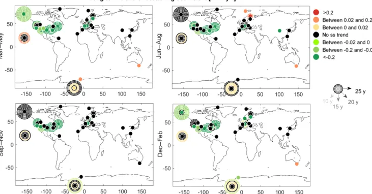
Abstract. In order to assess the evolution of aerosol parameters affecting climate change, a long-term trend analysis of aerosol optical properties was performed on time series from 52 stations situated across five continents. The time series of measured scattering, backscattering and absorption coefficients as well as the derived single scattering albedo, backscattering fraction, scattering and absorption Ångström exponents covered at least 10 years and up to 40 years for some stations. The non-parametric seasonal Mann–Kendall (MK) statistical test associated with several pre-whitening methods and with Sen’s slope was used as the main trend analysis method. Comparisons with general least mean square associated with autoregressive bootstrap (GLS/ARB) and with standard least mean square analysis (LMS) enabled confirmation of the detected MK statistically significant trends and the assessment of advantages and lim- itations of each method. Currently, scattering and backscattering coefficient trends are mostly decreasing in Europe and North America and are not statistically significant in Asia, while polar stations exhibit a mix of increasing and decreasing trends. A few increasing trends are also found at some stations in North America and Australia. Absorption coefficient time series also exhibit primarily decreasing trends. For single scattering albedo, 52 % of the sites exhibit statistically significant positive trends, mostly in Asia, eastern/northern Europe and the Arctic, 22 % of sites exhibit statistically significant negative trends, mostly in central Europe and central North America, while the remaining 26 % of sites have trends which are not statistically significant. In addition to evaluating trends for the overall time series, the evolution of the trends in sequential 10-year segments was also analyzed.

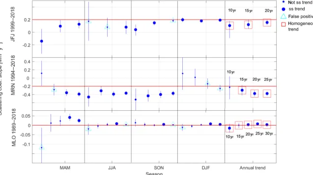
For scattering and backscattering, statistically significant increasing 10-year trends are primarily found for earlier periods (10-year trends ending in 2010–2015) for polar stations

and Mauna Loa. For most of the stations, the present-day statistically significant decreasing 10-year trends of the single scattering albedo were preceded by not statistically significant and statistically significant increasing 10-year trends.

The effect of air pollution abatement policies in continental North America is very obvious in the 10-year trends of the scattering coefficient – there is a shift to statistically significant negative trends in 2009–2012 for all stations in the eastern and central USA. This long-term trend analysis of aerosol radiative properties with a broad spatial coverage provides insight into potential aerosol effects on climate changes.

1 Introduction

Climate change has been considered a premier global prob- lem in the scientific community for decades. Thirty years ago, the community organized to produce the first Intergov- ernmental Panel on Climate Change (IPCC) report (IPCC, 1990) about the state of scientific, technical and socio- economic knowledge on climate change, its impacts and future risks, and options for reducing the rate at which climate change was taking place. Aerosols have been recognized as an important active climate forcing agent since the 1970s and, in the last IPCC report (IPCC, 2013), the impact of aerosols on the atmosphere was still considered to be one of the most significant and uncertain aspects of climate change projections and, for the first time, decadal trend analysis of in situ aerosol optical properties around the world was reported.

Aerosol optical properties are the relevant parameters that determine the radiative forcing of particulate matter. While some of these optical properties are currently measured by satellite (Choi et al., 2019), airborne and ground-based remote sensing (REM) technologies (https://aeronet.gsfc.nasa.

(3)

gov/, last access: 20 July 2020, https://www.earlinet.org/, last access: 20 July 2020), the ground-based, in situ measurements represent some of the longest time series, allowing assessment of the long-term time evolution of aerosol radiative properties in the lower troposphere.

The first in situ measurement network began in the mid 1970s at several remote locations (Bodhaine et al., 1995).

Through national and international programs and/or on an individual organization’s initiatives, the number of stations with systematic aerosol monitoring activities in regional background locations has continued to increase since the 1990s. As of 2017 absorption has been measured for at least 1 year (yr) at 50 sites, for 5 years at 37 sites and for 10 years at 20 sites, while scattering has been measured for at least 1 year at 56 sites, for 5 years at 45 sites and for 10 years at 30 sites. The companion paper (Laj et al., 2020) provides a historical view and a complete description of the present networks for aerosol measurements. The longest datasets cover up to 40 years of measurements, BRW (40 years), SPO (40 years), and MLO (31 years) (see Table 1 for station acronyms), whereas some stations with long time series recently closed or moved (THD, SGP, MUK, CPT). The spatial and temporal variability of aerosol properties is extremely high due to the short lifetime of aerosol particles (on the order of days to weeks), the wide variety of sources, as well as the chemical and microphysical processing occurring in the atmosphere; a dense network of stations is consequently re- quired to obtain a global view of aerosol changes. The grow- ing number of stations with long-term (>10 years) time series of aerosol particle optical properties – 24 in 2010 (Col- laud Coen et al., 2013, hereafter referred to as CC2013) and now 52 in 2016–2018 – is a positive factor. Detracting from that growth is the continued lack of sites in South America, Africa, Oceania and Asia.

Long-term measurements are the only possible approach for detecting change in atmospheric composition resulting from either changes in natural or anthropogenic emissions and/or changes in atmospheric processes and sinks. How- ever, detecting long-term trends of aerosol optical properties remains a challenge, due to their high natural variability, uncertainties caused by changes and biases in measurement methodology, the ill-defined statistical distribution of the parameters, the presence of high autocorrelation in aerosol parameters, as well as the occasional issues regarding trace- ability of historic operating procedures. Trend analysis can only be performed on time series without breakpoints or on homogenized time series that account for changes in measurement conditions (e.g., relocations, instrument calibration/repair/upgrades, inlet changes) (CC2013). Once homogenized datasets are available, appropriate techniques must be used to identify potential trends. The trend analysis methodology must take into account the non-normal distribution of most aerosol parameters, the high autocorrelation of the parameters, and the presence of gaps and negatives in the datasets.

In this current analysis, a considerable effort was made to detect time series breakpoints, to find explanations for them in the logbooks and station history and, if possible, to cor- rect or homogenize the time series. These homogenized time series were then subjected to an array of statistical tests to identify trends. These tests include (1) the non-parametric seasonal Mann–Kendall test (hereafter referred to as the MK test) associated with Sen’s slope. The applied MK test is however applied with a new pre-whitening method (Collaud Coen et al., 2020a), (2) a generalized least squares (GLS) method associated with a Monte Carlo bootstrap algorithm and (3) the least mean squares fit (LMS). While the MK test with pre-whitening was considered the most robust method, the other tests were included to allow a comparison between various simple and frequently used methods.

The first long-term trend analyses of aerosol optical properties, number concentration and particle size distribution (CC2013; Asmi et al., 2013) covered 2001–2010 as the short- est period and longer periods if data were available. The main observations were (1) a general statistically significant (ss) – at 95 % confidence level – decrease in number concentration, scattering and absorption coefficients in North America, (2) a ss decrease in number concentration in northeastern Eu- rope, (3) no ss trends in central Europe for any of the parameters and (4) no ss scattering coefficient trends but increasing 10-year absorption coefficient and number concentration trends in the polar regions. These trends were related to the decrease in anthropogenic primary aerosol emissions and in precursors of secondary aerosol formation. The high-altitude station Mauna Loa (MLO) in the Pacific was unique in ex- hibiting increasing optical property trends that were mostly attributed to long-range transport from Asia. The results in CC2013 are in line with the 1996–2013 trend analysis at the BND and SGP stations in North America (Sherman et al., 2015) showing a decreasing scattering coefficient and a sub-micron scattering fraction and increasing backscattering fraction. More recently, Pandolfi et al. (2018) presented the long-term trends of in situ surface aerosol particle optical properties (scattering) measured in Europe until 2015. The ss decreasing trends of aerosol particle scattering observed in Europe at around 40 % of the stations (mostly in Nordic and Baltic countries and southwestern Europe) were attributed to the implementation of continental to local emission mit- igation strategies. Pandolfi et al. (2018) also reported that the scattering Ångström exponent decreased at around 20 % for the European stations included in their study (at remote Nordic and Baltic locations and at two mountain sites in central and eastern Europe), whereas an increase was observed at 15 % of the stations (one urban site in southwestern Europe and one in central Europe). In the same study, the backscattering fraction was observed to increase. Trends in horizontal visibility synoptic observations over 1929–2013 from 4000 stations over the USA, Europe and Asia (Li et al., 2016) generally agreed with extinction coefficient trends, with a significant decrease in all regions but with different evolutions

(4)

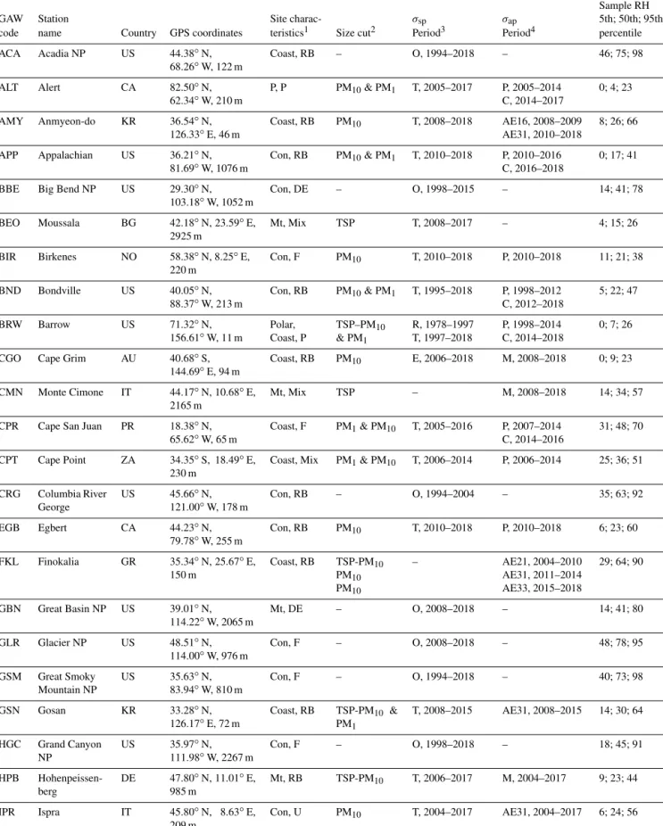
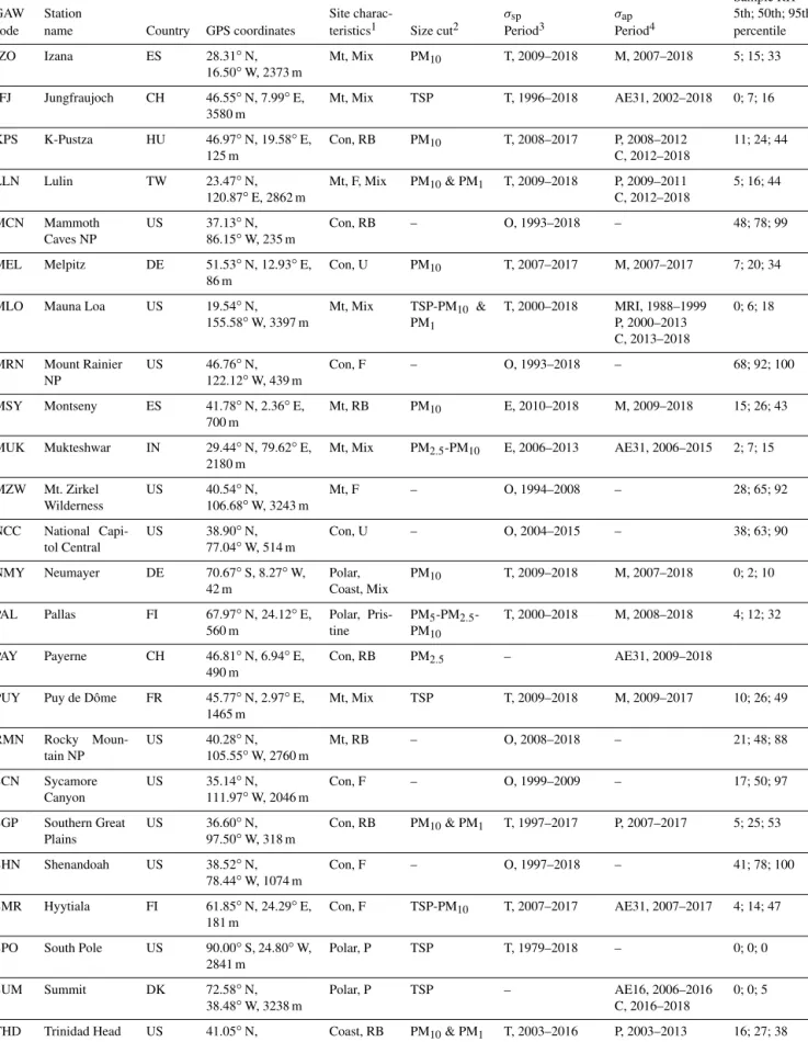
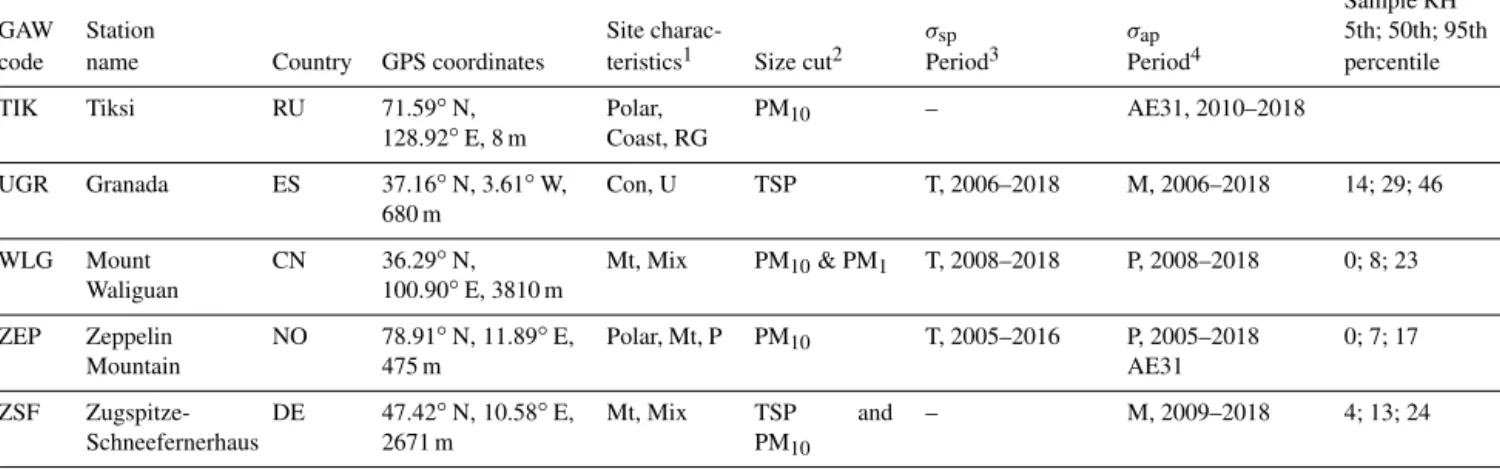
Table 1.List of observatories included in this study, arranged alphabetically by Global Atmospheric Watch (GAW) acronyms, including their names, countries, coordinates and elevation, site environmental characteristic (geographical category and footprint), size cut, type of nephelometer and absorption filter photometer deployed, time period used, and nephelometer RH percentiles.

Sample RH

GAW Station Site charac- σ_sp σ_ap 5th; 50th; 95th

code name Country GPS coordinates teristics¹ Size cut² Period³ Period⁴ percentile

ACA Acadia NP US 44.38^◦N,

68.26^◦W, 122 m

Coast, RB – O, 1994–2018 – 46; 75; 98

ALT Alert CA 82.50^◦N,

62.34^◦W, 210 m

P, P PM₁₀& PM₁ T, 2005–2017 P, 2005–2014 C, 2014–2017

0; 4; 23

AMY Anmyeon-do KR 36.54^◦N, 126.33^◦E, 46 m

Coast, RB PM₁₀ T, 2008–2018 AE16, 2008–2009 AE31, 2010–2018

8; 26; 66

APP Appalachian US 36.21^◦N, 81.69^◦W, 1076 m

Con, RB PM₁₀& PM₁ T, 2010–2018 P, 2010–2016 C, 2016–2018

0; 17; 41

BBE Big Bend NP US 29.30^◦N, 103.18^◦W, 1052 m

Con, DE – O, 1998–2015 – 14; 41; 78

BEO Moussala BG 42.18^◦N, 23.59^◦E, 2925 m

Mt, Mix TSP T, 2008–2017 – 4; 15; 26

BIR Birkenes NO 58.38^◦N, 8.25^◦E, 220 m

Con, F PM₁₀ T, 2010–2018 P, 2010–2018 11; 21; 38

BND Bondville US 40.05^◦N,

88.37^◦W, 213 m

Con, RB PM₁₀& PM₁ T, 1995–2018 P, 1998–2012 C, 2012–2018

5; 22; 47

BRW Barrow US 71.32^◦N,

156.61^◦W, 11 m

Polar, Coast, P

TSP–PM₁₀

& PM₁

R, 1978–1997 T, 1997–2018

P, 1998–2014 C, 2014–2018

0; 7; 26

CGO Cape Grim AU 40.68^◦S,

144.69^◦E, 94 m

Coast, RB PM₁₀ E, 2006–2018 M, 2008–2018 0; 9; 23

CMN Monte Cimone IT 44.17^◦N, 10.68^◦E, 2165 m

Mt, Mix TSP – M, 2008–2018 14; 34; 57

CPR Cape San Juan PR 18.38^◦N, 65.62^◦W, 65 m

Coast, F PM1& PM10 T, 2005–2016 P, 2007–2014 C, 2014–2016

31; 48; 70

CPT Cape Point ZA 34.35^◦S, 18.49^◦E, 230 m

Coast, Mix PM1& PM10 T, 2006–2014 P, 2006–2014 25; 36; 51

CRG Columbia River George

US 45.66^◦N, 121.00^◦W, 178 m

Con, RB – O, 1994–2004 – 35; 63; 92

EGB Egbert CA 44.23^◦N,

79.78^◦W, 255 m

Con, RB PM10 T, 2010–2018 P, 2010–2018 6; 23; 60

FKL Finokalia GR 35.34^◦N, 25.67^◦E, 150 m

Coast, RB TSP-PM10 PM₁₀ PM10

– AE21, 2004–2010

AE31, 2011–2014 AE33, 2015–2018

29; 64; 90

GBN Great Basin NP US 39.01^◦N, 114.22^◦W, 2065 m

Mt, DE – O, 2008–2018 – 14; 41; 80

GLR Glacier NP US 48.51^◦N, 114.00^◦W, 976 m

Con, F – O, 2008–2018 – 48; 78; 95

GSM Great Smoky Mountain NP

US 35.63^◦N, 83.94^◦W, 810 m

Con, F – O, 1994–2018 – 40; 73; 98

GSN Gosan KR 33.28^◦N,

126.17^◦E, 72 m

Coast, RB TSP-PM10 &

PM₁

T, 2008–2015 AE31, 2008–2015 14; 30; 64

HGC Grand Canyon NP

US 35.97^◦N, 111.98^◦W, 2267 m

Con, F – O, 1998–2018 – 18; 45; 91

HPB Hohenpeissen- berg

DE 47.80^◦N, 11.01^◦E, 985 m

Mt, RB TSP-PM10 T, 2006–2017 M, 2004–2017 9; 23; 44

IPR Ispra IT 45.80^◦N, 8.63^◦E,

209 m

Con, U PM10 T, 2004–2017 AE31, 2004–2017 6; 24; 56

(5)

Table 1.Continued.

Sample RH

IZO Izana ES 28.31^◦N,

16.50^◦W, 2373 m

Mt, Mix PM₁₀ T, 2009–2018 M, 2007–2018 5; 15; 33

JFJ Jungfraujoch CH 46.55^◦N, 7.99^◦E, 3580 m

Mt, Mix TSP T, 1996–2018 AE31, 2002–2018 0; 7; 16

KPS K-Pustza HU 46.97^◦N, 19.58^◦E, 125 m

Con, RB PM10 T, 2008–2017 P, 2008–2012 C, 2012–2018

11; 24; 44

LLN Lulin TW 23.47^◦N,

120.87^◦E, 2862 m

Mt, F, Mix PM10& PM1 T, 2009–2018 P, 2009–2011 C, 2012–2018

5; 16; 44

MCN Mammoth

Caves NP

US 37.13^◦N, 86.15^◦W, 235 m

Con, RB – O, 1993–2018 – 48; 78; 99

MEL Melpitz DE 51.53^◦N, 12.93^◦E, 86 m

Con, U PM10 T, 2007–2017 M, 2007–2017 7; 20; 34

MLO Mauna Loa US 19.54^◦N,

155.58^◦W, 3397 m

Mt, Mix TSP-PM₁₀ &

PM₁

T, 2000–2018 MRI, 1988–1999 P, 2000–2013 C, 2013–2018

0; 6; 18

MRN Mount Rainier NP

US 46.76^◦N, 122.12^◦W, 439 m

Con, F – O, 1993–2018 – 68; 92; 100

MSY Montseny ES 41.78^◦N, 2.36^◦E, 700 m

Mt, RB PM₁₀ E, 2010–2018 M, 2009–2018 15; 26; 43

MUK Mukteshwar IN 29.44^◦N, 79.62^◦E, 2180 m

Mt, Mix PM2.5-PM10 E, 2006–2013 AE31, 2006–2015 2; 7; 15

MZW Mt. Zirkel Wilderness

US 40.54^◦N, 106.68^◦W, 3243 m

Mt, F – O, 1994–2008 – 28; 65; 92

NCC National Capi- tol Central

US 38.90^◦N, 77.04^◦W, 514 m

Con, U – O, 2004–2015 – 38; 63; 90

NMY Neumayer DE 70.67^◦S, 8.27^◦W, 42 m

Polar, Coast, Mix

PM10 T, 2009–2018 M, 2007–2018 0; 2; 10

PAL Pallas FI 67.97^◦N, 24.12^◦E, 560 m

Polar, Pris- tine

PM5-PM2.5- PM₁₀

T, 2000–2018 M, 2008–2018 4; 12; 32

PAY Payerne CH 46.81^◦N, 6.94^◦E, 490 m

Con, RB PM_2.5 – AE31, 2009–2018

PUY Puy de Dôme FR 45.77^◦N, 2.97^◦E, 1465 m

Mt, Mix TSP T, 2009–2018 M, 2009–2017 10; 26; 49

RMN Rocky Moun- tain NP

US 40.28^◦N, 105.55^◦W, 2760 m

Mt, RB – O, 2008–2018 – 21; 48; 88

SCN Sycamore Canyon

US 35.14^◦N, 111.97^◦W, 2046 m

Con, F – O, 1999–2009 – 17; 50; 97

SGP Southern Great Plains

US 36.60^◦N, 97.50^◦W, 318 m

Con, RB PM₁₀& PM₁ T, 1997–2017 P, 2007–2017 5; 25; 53

SHN Shenandoah US 38.52^◦N,

78.44^◦W, 1074 m

Con, F – O, 1997–2018 – 41; 78; 100

SMR Hyytiala FI 61.85^◦N, 24.29^◦E, 181 m

Con, F TSP-PM₁₀ T, 2007–2017 AE31, 2007–2017 4; 14; 47

SPO South Pole US 90.00^◦S, 24.80^◦W, 2841 m

Polar, P TSP T, 1979–2018 – 0; 0; 0

SUM Summit DK 72.58^◦N,

38.48^◦W, 3238 m

Polar, P TSP – AE16, 2006–2016

C, 2016–2018

0; 0; 5

THD Trinidad Head US 41.05^◦N, 124.15^◦W, 107 m

Coast, RB PM₁₀& PM₁ T, 2003–2016 P, 2003–2013 C, 2013–2016

16; 27; 38

(6)

Table 1.Continued.

Sample RH

TIK Tiksi RU 71.59^◦N,

128.92^◦E, 8 m

Polar, Coast, RG

PM₁₀ – AE31, 2010–2018

UGR Granada ES 37.16^◦N, 3.61^◦W, 680 m

Con, U TSP T, 2006–2018 M, 2006–2018 14; 29; 46

WLG Mount

Waliguan

CN 36.29^◦N, 100.90^◦E, 3810 m

Mt, Mix PM10& PM1 T, 2008–2018 P, 2008–2018 0; 8; 23

ZEP Zeppelin Mountain

NO 78.91^◦N, 11.89^◦E, 475 m

Polar, Mt, P PM10 T, 2005–2016 P, 2005–2018 AE31

0; 7; 17

ZSF Zugspitze- Schneefernerhaus

DE 47.42^◦N, 10.58^◦E, 2671 m

Mt, Mix TSP and

PM₁₀

– M, 2009–2018 4; 13; 24

1Geographical category: Mountain: Mt, Polar: P, Continental: Con, Coastal: coast. Footprint: Rural background: RB, Forest: F, Desert: DE, (Sub-)Urban: U, Pristine: P Mixed: Mix.

2the mention of two size cuts separated by “–” corresponds to a modification of inlet during the tim series, whereas the “&” corresponds to measurements at two size cuts.

3T: TSI nephelometer, O: Optec nephelometer, R: Radiance Research nephelometer; E3: Ecotech nephelometer Aurora 3000, E4: Ecotech nephelometer Aurora 4000.

4AE16(Cref=1.8) 120/AE22 (Cref=1.8)/AE31 (Cref=3.5)/AE33 (Cref=3.5): Aethalometer, P1: one-wavelength or P3: three-wavelength PSAP, M: MAAP, C: NOAA CLAP, ET: ES95L Thermo 5012==M.

of the trends. Hand et al. (2014) also found a significant drop of the ambient light extinction coefficient at all IM- PROVE (Interagency Monitoring of Protected Visual Envi- ronment, http://vista.cira.colostate.edu/Improve/, last access:

20 July 2020) stations over the 1990s through 2011, with a larger decrease in the eastern USA. To our knowledge, no further trend analyses of surface in situ aerosol optical properties involving a network of stations or several stations have been published up to now.

This study is part of the SARGAN (in-Situ AeRosol GAW observing Network) initiative (see the companion paper by Laj et al., 2020) with the objective of supporting a global aerosol monitoring network to become a GCOS (Global Cli- mate Observing System) associated network. This trend analysis is intended to answer the following questions.

1. Are there homogeneous long-term trends of in situ aerosol optical properties over the covered regions of the world? Do they differ as a function of the length of the data series? How do the trends evolve with time?

2. Are there regional similarities or differences in the observed trends among stations? Are there similarities or differences in trends among aerosol parameters at regional and continental scales?

3. How do the observed optical property trends compare with trends in other aerosol and gaseous properties reported in the literature?

The results of this study provide the best representation of change in surface aerosol optical properties considering the available in situ aerosol optical property datasets and high- light the possible side-effects of air pollution control policies on radiative forcing.

2 Experimental 2.1 Measurement sites

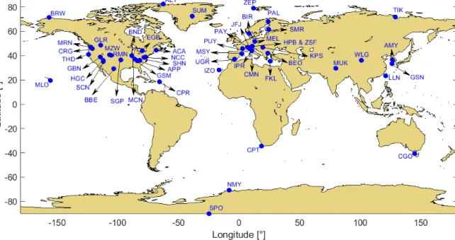
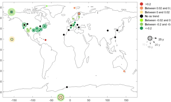
The long-term trend analysis presented in this study ana- lyzes in situ aerosol time series from 52 observatories world- wide shown in Fig. 1 with site information listed in Table 1.

The network, which is a subset of the station network described in Laj et al. (2020), comprises 16 stations in Europe, 21 in North America, 5 in Asia, 2 in Africa, 6 in the polar regions and 2 in the southwestern Pacific. The stations included in this study are primarily located in rural or remote areas and are expected to exhibit regional- to large- scale representativeness (e.g., Wang et al., 2018). Apart from MUK, all the stations are regional or global GAW (Global Atmospheric Watch, https://gawsis.meteoswiss.ch/GAWSIS/

/index.html#/, last access: 20 July 2020) sites or IMPROVE stations. The GAW aerosol data are archived at and available from the World Data Centre for Aerosol (WDCA, http://

www.gaw-wdca.org, last access: 20 July 2020) located at the Norwegian Institute for Air Research (NILU). The WDCA data repository is the EBAS database (http://ebas.nilu.no, last access: 20 July 2020), an e-infrastructure shared with other frameworks targeting atmospheric aerosol properties, such as the Co-operative Programme for Monitoring and Evaluation of the Long-range Transmission of Air pollu- tants in Europe (EMEP) and the European Aerosols, Clouds, and Trace gases Research InfraStructure Network (ACTRIS).

The IMPROVE data are available from the IMPROVE web- site (http://vista.cira.colostate.edu/Improve/data-page/, last access: 20 July 2020) and from the WDCA. To ensure that the long-term trend analysis was performed on homogeneous time series, a substantial effort of quality control, rupture de- tection and homogenization (see Sect. 2.4) was performed in close collaboration with each station’s operator on the data.

(7)

Figure 1.Map of stations with their GAW acronyms.

As has been noted in previous papers, it is critical to have outside review of data to improve the quality of long-term time series (CC2013; Asmi et al., 2013). The final time series used in this analysis are available from the following DOI:

https://doi.org/10.21336/c4dy-yw57.

The stations’ environments were classified into four types (continental, coastal, mountain, or polar) that are represented by 22, 8, 16 and 7 time series, respectively. The type of measured aerosol at each site is further characterized by their footprints comprising six types (rural background, forest, desert, (sub)-urban, pristine and mixed). While the environments of Europe, North America and the polar regions are fairly well represented, the number of long-term stations in the rest of the world is currently quite low, resulting in a lack of information from the largest deserts (e.g., Sahara, Gobi, Australian, Arabian, Atacama), from many mountain ranges (e.g., Himalaya, Andes, Southern Great Escarpment, Great Dividing Range, Urals) and from whole continents (South America (no site), Africa (one island in the Atlantic and one coastal site), and Australia (one coastal site)). Some stations from these underrepresented areas currently have 4 to 7 years of measurements available and will potentially be used for trend analyses in the future (see Table 3 in Laj et al., 2020).

Sites were chosen based on the following criteria:

(1) availability of at least 10 years of continuous data (two sites with 9 years and one site with 8 years of data for at least one parameter have also been included to improve spatial coverage (CPT, EGB and GSN, respectively)); (2) continuous measurements without ruptures in the aerosol light scattering and/or absorption measurement; (3) submission of quality-assured data to the WMO WDCA data repository;

and (4) responsiveness of site operators to questions concern- ing data quality and homogeneity.

The longest time series with 40 years of measurements are the Arctic and Antarctic stations of BRW and SPO, fol- lowed by the high-altitude MLO station (31 years). During the 1990s NOAA began extending their network (Andrews et al., 2019), the IMPROVE network installed numerous stations in the USA (Malm et al., 1994), and the first long-term measurements in Europe, JFJ (Bukowiecki et al., 2016) and HPB, began in 1995. To have the largest representativity and to minimize the number of stations with less than 10 years of measurement, the current long-term trends were computed from time series ending in 2016, 2017 or 2018 (whichever year was most recently available). To obtain an overview of the long-term trend evolution in the past 40 years, all stations with at least 10 years of measurements were considered (see results in Sect. 3.2).

2.2 Instruments

The relevant instruments operating at each site are listed in Table 1 and further instrument details are given in the Supple- ment (Table S1). Some particular instrumental features that could influence the trend analysis or comparison between stations are briefly discussed below.

Nephelometers measure aerosol light scattering over a truncated angular range (Müller et al., 2009, and references therein), leading to non-idealities often called “truncation er- ror”. The truncation adjustment accounts for scattering over the angles outside the measurement range and non-ideality of the light source. All TSI nephelometer scattering and backscattering sets were adjusted for truncation and instru-

(8)

ment non-idealities using the Anderson and Ogren (1998) correction. Thus, for times when enhanced amounts of large diameter (D_p>1 µm) particles are present, the measured scattering will be lower than true scattering by a substantial amount since the truncation correction increases with particle size (Anderson and Ogren, 1998; Molenar et al., 1997).

The Radiance Research nephelometer has similar truncation characteristics to the TSI nephelometer (Müller et al., 2009). The Optec nephelometer measures over a wider angular range (Molenar, 1997) than the other nephelometers and, like the Radiance Research measurements, the scattering has not been corrected for truncation in this study. The Optec nephelometers measure at ambient conditions with no size cut (they are open-air instruments) so they can sample the very large particles present due to both hygroscopic growth at high humidities and/or the occurrence of precipitation, fog, dust, pollen, etc. The Ecotech nephelometers have a similar angular range to the TSI nephelometers, and the measurements are corrected for truncation errors using the Müller correction (Müller et al., 2011b), adapted from the Anderson and Ogren correction.

For better comparability of aerosol properties amongst sites and to minimize the confounding effects of water associated with the aerosol, GAW recommends drying the sample air to RH<40 % (WMO/GAW report 227, 2016). While most of the nephelometer scattering time series are accompa- nied by sample RH measurements, this was not the case for all stations and for the entire measurement period. The calculated RH trends are therefore not always complete. Many breakpoints were detected in sample RH data and exchanges with the individual station operators revealed that humidity sensors often suffer from artifacts, offsets, and modifications that were not considered problematic. These sensor problems were often not resolved due to the secondary status of this housekeeping diagnostic, leading to problematic time series.

Nonetheless, apart from the IMPROVE network, the majority of nephelometers appeared to have sampled at RH<40 %.

The IMPROVE scattering measurements were analyzed at the measurement conditions with some constraints on ac- ceptable scattering values, although the IMPROVE network recommends screening the data when RH>90 % (Prenni et al., 2019). For this study and according to CC2013, the IM- PROVE scattering coefficient was restricted to σsp values lower than 500 M m⁻¹for stations in the eastern USA (ACA, GSM, MCN and SHN) and lower than 100 M m⁻¹ for stations in the western USA to minimize the influence of rain, fog, snow and ice. These screening constraints minimized the issues associated with high RH but do not correspond to a screening based on RH.

Measurement of the absorption coefficient was always performed by some type of filter-based photometer but relied on a variety of instruments. These instruments include Multi- Angle Absorption Photometers (MAAPs), Particle Soot Ab- sorption Photometers (PSAPs) and Continuous Light Ab- sorption Photometers (CLAPs), as well as various models

of the Aethalometer (AE16, AE21, AE31 and AE33). All these instruments suffer from various artifacts, from which the loading effect can influence the wavelength dependence.

However, the largest uncertainty in filter-based photometer measurements lies in the effect of the multiple scattering of light into the filter matrix, leading to over-prediction of absorption aerosol (e.g., Bond et al., 1999; Lack et al., 2008;

Müller et al., 2011a; Collaud Coen et al., 2010; Bernardoni et al., 2019). This artifact is roughly corrected by the multiple scattering constantC_refand is probably largest for the Aethalometer and smallest for the MAAP.

The ACTRIS community has suggested that Level 2 AE31 data submitted to EBAS utilize a multiple scattering constant Cref=3.5; most of the analyzed AE31 time series were corrected with this new rule. The AE33 adds a simultaneous measurement of the light transmission through a second filter spot sampling the same air at a different flow rate associated with a real-time compensation algorithm. This two-spot technique allows for correction of the filter loading artifact.

This improvement, however, has no effect on the largest artifact (multiple scattering artifact) and, as of yet, there is no agreed upon correction for the AE33 by the aerosol community. Previous AE models used a white light diode (AE10 and AE16) and aC_ref=1.6 is usually applied. At FKL, the AE21 used aC_ref=1.8 and the AE33 aC_ref=3.0. The various ver- sions of the Aethalometer require then different corrections, whereas the realCrefvalue depends on the filter and on the aerosol type. For background rural aerosol, the realCrefvalue is between 2.5 and 4.5 (Collaud Coen et al., 2010; Bernar- doni et al., 2019), the Asian plume has a relatively highCref

between 4 and 5.5 (Kim et al., 2018), in the ArcticCref is suggested to be 3.45 (Backman et al., 2017), whereas pure mineral dust leads to a lowerCrefof 1.75–2.56 (Di Biagio et al., 2017).

The MAAP measures not only the light transmission through the filter, but also the light backscattered at two different angles. This design takes into account the scattering and multiple scattering artifacts (see Collaud Coen et al., 2010), which are two of the most significant artifacts for filter-based absorption photometers so that no correction is needed (C_ref=1). The MAAP measured absorption coefficient is consequently more reliable.

The CLAP was developed by NOAA as a replacement for the PSAP (Ogren et al., 2017). The CLAP was designed to have the same optical characteristics as the PSAP so that either the Bond et al. (1999) correction along with the Ogren (2010) update for wavelength and spot size correction or the Virkkula et al. (2005, 2010) corrections can be applied to account for scattering artifacts at multiple wavelengths as well as other instrument non-idealities (e.g., filter-loading artifacts, variability in spot size and flow calibrations). These correction algorithms rely on co-located scattering measurements from a nephelometer and may have issues in the presence of large, primarily scattering aerosol such as sea salt or

(9)

dust (e.g., Bond et al., 1999) and also may not work well when organic aerosol is abundant (e.g., Lack et al., 2008).

The differences in instrumentation, measurement conditions and post-processing data treatment do not allow the absolute values of aerosol optical parameters for all sites to be compared; however, because there was consistency of data treatment for each individual time series, the trends across the different sites can be compared.

2.3 Aerosol optical properties

The data used in this paper consist of hourly-averaged, quality-checked, spectral light scattering (σsp), backscattering (σ_bsp) and absorption (σ_ap) measurements. The quality checks correspond to the Level 2 requirements of EBAS (Laj et al., 2020). After further visual quality control by the au- thors, the hourly data were aggregated into daily medians with the requirement that at least 25 % of the daily data be valid. The median was chosen to minimize the effect of extreme values on the average since the measured parameters are strongly not normally distributed and most of the calculated parameters also do not follow a normal distribution. Such a low requirement for data coverage was chosen since six hourly measurements a day corresponds to half of the potential data coverage at many of the NOAA stations, where the operation mode consists of alternating between PM1and PM10 size cutoff on a sub-hourly basis (Andrews et al., 2019).

All the nephelometers and the multi-wavelength absorption photometers measure at a green wavelength (∼525–

550 nm), which is the channel for which the parameters are reported. For the AE31 and AE33 models, the 520 nm channel was chosen. At several sites, the light absorption was measured by white light (∼840–880 nm) Aethalome- ters (AE16), two-channel Aethalometers (AE21) using 370 and 880 nm or by MAAPs (Multi-Angle Absorption Pho- tometers) at 637 nm (Müller et al., 2011a), requiring the use of another wavelength, typically a red wavelength. In some cases, the blue or red wavelength was preferred due to inhomogeneities or gaps in the green data. Since the trend analysis is not sensitive to the multiplication by a constant, the data series used to determine scattering and absorption trends were not adjusted to 550 nm.

In addition to the measured parameters, the following parameters were computed when the appropriate measurements were available:

– backscatter fraction,b=σ_bsp/σ_sp, – scattering Ångström exponent,

å_sp= −ln(σ_sp,1/σ_sp,2)/ln(λ₁/λ₂), – absorption Ångström exponent,

å_ap= −ln(σ_ap,1/σ_ap,2)/ln(λ₁/λ₂), or by a linear fit between the logarithm of the seven absorption coefficients as a function of the logarithm of the seven wavelengths of the Aethalometers (AE31 and AE33), and

– single scattering albedo,ω0=σsp/(σsp+σap), whereσsp,i is the scattering coefficient at wavelengthi,λi

is the wavelengthi,σbsp is the hemispheric backscattering coefficient, andσapis the absorption coefficient.

å_sp and å_ap were usually computed from the blue (∼450 nm) and green wavelengths, because the red channel of the nephelometers was frequently less stable and more prone to rupture in the time series due to calibrations or instrument changes. However, in some cases, other wavelength pairs were used to utilize the longest time series. å_apcom- puted from AE31 and AE33 is always more homogeneous if fitted on the seven wavelengths, so that the fitted å_apwas always chosen for these two instruments.

The single scattering albedo was computed fromσsp and σapafterσapwas adjusted to match the nephelometer green wavelength with an assumed absorption Ångström exponent of one (i.e., 1/λdependence). In order to maintain similar data treatment for absorption instruments with single or multiple wavelengths, the measured absorption Ångström exponents were not used for the wavelength adjustment for theω₀ calculation.

It should be recalled that all parameters calculated using ratios of theσ_sp,σ_bspand/orσ_apmay have higher uncertainties for two reasons: (1) the ratio of two similar values has a larger uncertainty than theσ_sp,σ_bsporσ_apuncertainties and (2) theσ_spdifference between the wavelengths depends on the nephelometer calibration that is performed independently for each wavelength. These uncertainties are particularly enhanced for clean locations with low aerosol loading.

2.4 Discontinuities, data consistency and homogenization

Long-term climate analyses require homogeneous time series to be accurate. A homogeneous climate time series is defined as one where variations are caused only by variations in weather and climate (Conrad and Pollak, 1950) and in emissions of aerosol particles and their precursor gases. Long- term climatological time series can be affected by a number of non-climatic factors called breakpoints (e.g., reloca- tion, instrument upgrades, inlet changes, calibrations, nearby pollution sources) that mask the real climate variations. The breakpoints can be detected either by subjective visual inspection or by objective statistical methods (Peterson et al., 1998; Beaulieu et al., 2007) and must correspond to an event recorded in logbooks describing the station/instrumental history. Many statistical methods are only suitable for normally distributed data and cannot therefore be applied to aerosol optical property measurement without data transformation (Lindau and Venema, 2018). Moreover, they are often applied not only to the data, but also to ratios or differences between various time series that are not systematically available at all the measuring sites of this study.

Visual inspection was used to detect breakpoints and to assess the validity of the time series to be used for climatic

(10)

trend analysis. For this study, each measured and calculated (see Sect. 2.3) parameter at all wavelengths, as well as all the possible ratios between measured parameters (including the number concentration if available), at each station were visually inspected in linear and logarithmic time series plots. The treatment of minimum and maximum values, outliers and negatives along with the consistency of seasonal cycles were looked at closely when inspecting the time series plots. In addition, the data owners responded to a questionnaire about potential breakpoints, providing metadata that could be used to confirm/dismiss possible breakpoints or to accurately lo- cate them. The identified breakpoints were discussed with the data owners, leading to corrections, homogenization, in- validations or splitting of the time series into two parts. In one case (absorption data from SUM measured by AE16 and CLAP), the two time series were homogenized by multiply- ing the AE16 data by the median of the ratio between both datasets during the 10.5 months of simultaneous measurements. Only datasets considered homogeneous by the au- thors and the data owners were analyzed in this study.

In the older networks, several modifications likely lead to inhomogeneities that occurred at sites in the network around the same time. Some of these include the following.

1. Two of the longest running NOAA stations changed their TSP (total suspended particle) inlets for PM₁₀ size cuts in the middle of the multi-decade time series (MLO: 2000, BRW: 1997). Some other stations outside the NOAA network also modified the measurement size cuts over their long-term measurement period. Usually this change in size cut (TSP to PM10) did not generate a breakpoint for aerosol optical properties so that the time series could be considered homogeneous. A differ- entiation between periods of sampling inside or outside of clouds was not made, even though TSP and PM₁₀ could respond differently in these situations. In contrast, the modification of TSP or PM₁₀ size cuts to PM_2.5 or PM₁cutoffs usually led to visible breakpoints. PAL is the only station where changes between PM₁₀, PM₅ and PM_2.5did not induce a visually obvious breakpoint, likely due to the minimal presence of supermicron particles at this site.

2. The NOAA stations used the single green wavelength PSAP until the years 2005–2007, when they replaced them with a three-wavelength (3w) PSAP (see Ta- ble S1). This instrumental change usually did not induce a visually obvious breakpoint.

3. A further instrument change for the absorption coefficient at NOAA sites occurred in 2013–2015 through the introduction of the 3w CLAP. The 3w PSAP to 3w CLAP change usually induced no breakpoint in the green absorption coefficient. The red channel some- times exhibited a visible breakpoint (APP and BND), resulting in breakpoints in the absorption Ångström ex-

ponent. In those cases, calculation of the absorption Ångström exponent with the blue and green channels was preferred.

4. The long time series from MLO and JFJ were subject to the removal of negative values during the first years of measurements until 2000 and 1999, respectively. The raw data prior to these years were not archived by the data providers for either site. This change in minimal values does not seem to produce a clear breakpoint in the sense that the computed trends were not affected strongly enough to modify the climatic trends.

To compare long-term trends between stations from various networks, instruments and operators, instrumentation, measurement conditions and data treatment consistency is critical, but some lenience amongst stations was deemed ac- ceptable. Specifically, some discretion was allowed, including whether the datasets had the same corrections applied (e.g., truncation or not), how the sites dealt with sample RH and very low aerosol amounts, and inlet size cuts. Table 1 includes columns indicating information about the size cuts and RH conditions at the various sites. No screening or analysis as a function of cloud amount/clear-sky conditions was done since these criteria/flagging were not available at all stations. Below, the impacts of sample RH, size cut and general instrument conditions and corrections on trend evaluation are briefly discussed.

1. Humidity: one important factor affecting all aerosol measurements is the relative humidity (RH) at which the measurements are made. Forσsp, measurements at controlled RH enable minimization of the confounding effects of aerosol hygroscopic growth, resulting in increases in the amount of scattering aerosol (Nessler et al., 2005; Fierz-Schmidhauser et al., 2010; Burgos et al., 2019). The disadvantage of making measurements at low RH is that aerosol hygroscopic properties must be measured or assumed in order to adjust the aerosol optical properties to ambient conditions. As noted above (see Sect. 2.2), within the GAW program, recommendations have been given to measureσ_spat low (RH<40 %) humidities. Apart from the IMPROVE and CPR nephelometers, the instruments typically operated at RH<50 %, with only six stations having a RH 95th percentile value larger than 50 % (AMY, CMN, EGB, GSN, IPR and SGP) but with a median clearly much lower than 50 %. In contrast, the IMPROVE network instruments measure at near-ambient conditions (Malm et al., 1996). The scattering restriction method (see Sect. 2.2) was chosen in order to maintain the highest data coverage – simply removing scattering values associated with RH>50 % from the ambient IMPROVE dataset would have eliminated most of the summertime measurements, particularly for the eastern USA locations. For all stations with some contribution of scatter-

(11)

ing made at RH values larger than 50 %, the dry scattering and backscattering coefficients were calculated by removing values corresponding to hourly RH median>50 %.

Ensuring a low humidity in the nephelometer reduces but does not suppress the potential influence of the hygroscopic growth on nephelometer measurements (Zieger et al., 2013). Therefore, if RH data were available, the RH long-term trends were also computed and their potential effect on the trend ofσ_sp,σ_bsp,band å_sp was evaluated (see Sect. 4.1).

The filter-based absorption photometers are also sensitive to rapid RH changes (e.g., Anderson et al., 2003), but daily absorption averages are usually not biased by such rapid fluctuations (Bernardoni et al., 2019).

Very high sample RH could lead to higher uncertainties, but absorption measurements at GAW stations are usually connected to inlets with some sort of condi- tioning intended to reduce sample RH (e.g., diffusion or membrane dryers, dilution with dry air and, in some cases, heating). Additionally, CLAPs are gently heated to∼37^◦C to minimize RH effects. In this study, stations with high sample RH in the nephelometer sample (Table 1) are also the most likely to have issues with high sample RH in the collocated absorption photometer.

2. Size cut: as described in Table 1, the size cuts differ amongst the stations, but most of the sites measure TSP or PM10. The GAW program generally recommends a PM10 size cut, except for stations in extreme environments (clouds, etc.), where a whole air inlet is recom- mended (WMO/GAW report 227, 2016; GAW/WCCAP recommendations https://www.wmo-gaw-wcc-aerosol- physics.org/files/WCCAP-recommendation-for- aerosol-inlets-and-sampling-tubes.pdf, last access:

20 July 2020). Many stations in the NOAA Federated Aerosol Network measure at a second size cut (PM₁) as well. PAY and SUM are the only stations that have no measurement of coarse-mode aerosol, with only a PM_2.5 inlet. As reported previously, the amount of aerosol particles larger than 10 µm is usually suffi- ciently low to enable consideration of TSP and PM10

results as being in the same category. Moreover, the trend results of PM10 and PM1 sampling are found to be quite similar for all stations with both size cuts, so that the results of TSP/PM₁₀size cut will be presented in this study and, if not specified, PM₁results can be assumed to be similar to those of the larger size cut (PM₁₀or TSP).

3. Absorption filter photometer artifacts: the first main point to consider is that all filter-based absorption photometers suffer from various measurement artifacts and that continuous reference measurements to assess the

absoluteσapvalues are not available at long-term monitoring sites. If the variability and the long-term trends of absorption coefficients are to be analyzed with high confidence, theσ_apabsolute value is necessary to com- pute theω₀. As stated in Sect. 2.2, the realC_refvalues can potentially vary by a factor of 4 (1.5 to 5.5). Us- ing an erroneous C_ref value can influence the magni- tude of theω₀ trends. Similarly, an applied correction depending on the wavelengths can affect the absorption Ångström exponent calculation and its trends. Bothω₀ and å_aplong-term trends therefore must be interpreted with greater care.

4. Nephelometer truncation correction artifacts: as ex- plained in Sect. 2.2, the various types of nephelometers measure at different truncated angular ranges that were corrected by several algorithms or even not corrected.

The absence of truncation correction leads to lower scattering and backscattering coefficients than the true values and the correction algorithm effects are known to increase with particle size. The most important requirement that was verified for this trend analysis is the co- herent treatment of nephelometer data for each time series. The bias leading to a higher contribution of Aitken and accumulation modes than the coarse mode is dif- ficult to estimate, but the minimal differences in PM₁ and PM10 results (see Sect. 4.2) suggest this artifact is small. The effect of the humidity on the nephelometer measurements is regarded as the most significant artifact.

Finally, in order to minimize the potential artifacts in the de- termination of the long-term trends in the case of large seasonal variability (de Jong and de Bruin, 2012), only full start and end years of the time series, that is, without gaps in the data, were considered. For some stations, we did allow gaps of up to 4–6 weeks without measurements after checking that the removal of the whole year led to similar trend results.

The differences in instrumentation, measurement conditions, and post-processing data treatment do not allow the absolute values for all sites to be compared; however, because there was consistency of data treatment for individual sites, the trends can be compared.

2.5 Trend analyses

The aerosol extensive parameters (σsp, σbsp and σabs) are not normally distributed and they exhibit varying degrees of autocorrelation. They can be represented approximately by a lognormal distribution but are usually better fitted by a distribution in the Johnson distribution family (Johnson, 1949). The intensive parameters (b, å_sp, å_apandω₀) also exhibit distributions that differ to varying degrees from the normal distribution. We chose, therefore, to rely mostly on the non-parametric seasonal Mann–Kendall (MK) test associated with Sen’s slope. The MK test does not require normally