Portfolio solver for verifying Binarized Neural Networks
Gergely Kovásznai
a, Krisztián Gajdár
b, Nina Narodytska
caEszterházy Károly University, Eger, Hungary kovasznai.gergely@uni-eszterhazy.hu
bEricsson Hungary, Budapest, Hungary
cVMware Research, Palo Alto, USA Submitted: November 21, 2020
Accepted: March 17, 2021 Published online: May 18, 2021
Abstract
Although deep learning is a very successful AI technology, many concerns have been raised about to what extent the decisions making process of deep neural networks can be trusted. Verifying of properties of neural networks such as adversarial robustness and network equivalence sheds light on the trustiness of such systems. We focus on an important family of deep neural networks, the Binarized Neural Networks (BNNs) that are useful in resource- constrained environments, like embedded devices. We introduce our portfolio solver that is able to encode BNN properties for SAT, SMT, and MIP solvers and run them in parallel, in a portfolio setting. In the paper we propose all the corresponding encodings of different types of BNN layers as well as BNN properties into SAT, SMT, cardinality constrains, and pseudo-Boolean constraints. Our experimental results demonstrate that our solver is capable of verifying adversarial robustness of medium-sized BNNs in reasonable time and seems to scale for larger BNNs. We also report on experiments on network equivalence with promising results.
Keywords:Artificial intelligence, neural network, adversarial robustness, for- mal method, verification, SAT, SMT, MIP
doi: https://doi.org/10.33039/ami.2021.03.007 url: https://ami.uni-eszterhazy.hu
183
1. Introduction
Deep learning is a very successful AI technology that makes impact in a variety of practical applications ranging from vision to speech recognition and natural language [17]. However, many concerns have been raised about the decision-making process behind deep learning technology, in particular, deep neural networks. For instance, can we trust decisions that neural networks make [14, 18, 32]? One way to address this problem is to define properties that we expect the network to satisfy. Verifying whether the network satisfies these properties sheds light on the properties of the function that it represents [7, 23, 31, 34, 37].
One important family of deep neural networks is the class ofBinarized Neural Networks (BNNs) [20]. These networks have a number of useful features that are useful in resource-constrained environments, like embedded devices or mobile phones [25, 28]. Firstly, these networks are memory efficient, as their parameters are primarily binary. Secondly, they are computationally efficient as all activations are binary, which enables the use of specialized algorithms for fast binary matrix multiplication. Moreover, BNNs allow a compact representation in Boolean logic [7, 31].There exist approaches that formulate the verification of neural networks to Satisfiability Modulo Theories (SMT) [13, 19, 23], while others do the same to Mixed-Integer Programming (MIP) [11, 15, 36]. In some sense, this work can be considered to be the continuation of that in [7, 31], which translate all the MIP constraints to SAT.
The goal of this work to attack the problem of verifying important properties of BNNs by applying several kinds of approaches and solvers, such asSAT, SMT and MIP solvers. We introduce our solver that is able to encode BNN properties for those solvers and run them in parallel, in a portfolio setting. We focus on the important properties of neural networks adversarial robustness and network equivalence.
In this paper we introduce how to use our solver and report on experiments on verifying both robustness and equivalence. Experimental results show that our solver is capable of verifying those properties of medium-sized BNNs in reasonable runtime, especially when the solversMiniCARD+Z3are run in parallel.
2. Preliminaries
A literal is a Boolean variable 𝑥 or its negation ¬𝑥. A clause is a disjunction of literals. A Boolean formula is in Conjunctive Normal Form (CNF), if it is a conjunction of clauses. We say that a Boolean formula, typically in CNF, is satisfiable, if there exists a truth assignment to the Boolean variables of the formula such that the formula evaluates to 1 (true). Otherwise, it is said to beunsatisfiable (UNSAT). TheBoolean Satisfiability (SAT)problem is the problem of determining if a Boolean formula is satisfiable.
Satisfiability Modulo Theories (SMT)is the decision problem of checking satis-
fiability of a Boolean formula with respect to some background theory. Common theories include the theory of integers, reals, fixed-size bit-vectors, etc. The logics that one could use might differ from each other in the linearity or non-linearity of arithmetic and the presence or absence of quantifiers. In this paper, we use the theory of integers combined with linear arithmetic and without quantifiers – denoted asQF_LIAin the SMT-LIB standard [5].
ABoolean cardinality constraint is defined as an expression∑︀𝑛
𝑖=1𝑙𝑖 ∘rel𝑐, where 𝑙1, . . . , 𝑙𝑛 are literals, ∘rel∈ {≥,≤,=}, and𝑐∈Nis a constant where0≤𝑐≤𝑛.
A pseudo-Boolean constraint can be considered as a “weighted” Boolean car- dinality constraint, and can be defined as an expression ∑︀𝑛
𝑖=1𝑤𝑖𝑙𝑖 ∘rel𝑐, where 𝑤𝑖∈N,𝑤𝑖>0.
We assume the reader is familiar with the notion and elementary properties of feedforward neural networks. We consider a feedforward neural network to compute a function𝐹 where𝐹(𝑥)represents the output of𝐹on the input𝑥. Letℓ(𝑥)denote the ground truth label of𝑥. Our tool can analyze two properties of neural networks:
adversarial robustness and network equivalence. We call a neural network robust on a given input if small perturbations to the input do not lead to misclassification, as defined as follows, where𝜏 represents the perturbation and𝜖∈Nthe upper bound for the𝑝-norm of 𝜏.
Definition 2.1(Adversarial robustness). A feedforward neural network𝐹 is(𝜖, 𝑝)- robust for an input𝑥if¬∃𝜏,‖𝜏‖𝑝≤𝜖such that𝐹(𝑥+𝜏)̸=ℓ(𝑥).
The case of𝑝=∞, which bounds the maximum perturbation applied to each entry in𝑥, is especially interesting and has been considered frequently in literature.
Similar to robustness, the equivalence of neural networks is also a property that many would like to verify. We consider two neural networks equivalent if they generate the same output on all inputs, as defined as follows, where𝒳 denotes the input domain.
Definition 2.2 (Network equivalence). Two feedforward neural networks 𝐹1 and 𝐹2 are equivalent if∀𝑥∈ 𝒳 𝐹1(𝑥) =𝐹2(𝑥).
3. Encoding of Binarized Neural Networks
A Binarized Neural Network (BNN) is a feedforward network where weights and activations are predominantly binary [20]. It is convenient to describe the structure of a BNN in terms of composition of blocks of layers rather than individual layers.
Each block consists of a collection of linear and non-linear transformations. Blocks are assembled sequentially to form a BNN.
Internal block. Each internal block (denoted asBlock) in a BNN performs a collection of transformations over a binary input vector and outputs a binary vector.
While the input and output of a Blockare binary vectors, the internal layers of Block can produce real-valued intermediate outputs. A common construction
of an internal Block (taken from [20]) is composed of three main operations:1 a linear transformation (Lin), batch normalization (Bn), and binarization (Bin).
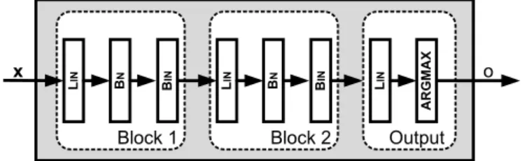
Table 1 presents the formal definition of these transformations. Figure 1 shows two Blocks connected sequentially.
LIN BN BIN
x
Block 1
LIN BN BIN
Block 2
LIN ARGMAX
Output o
Figure 1. A schematic view of a binarized neural network. The internal blocks also have an additionalHardTanhlayer during the
training.
Table 1. Structure of internal and outputs blocks which stacked to- gether form a binarized neural network. In the training phase, there might be an additionalHardTanhlayer after batch normalization.
𝐴𝑘and𝑏𝑘are parameters of theLinlayer, whereas𝛼𝑘𝑖, 𝛾𝑘𝑖, 𝜇𝑘𝑖, 𝜎𝑘𝑖
are parameters of theBnlayer. The𝜇’s and𝜎’s correspond to mean and standard deviation computed in the training phase. TheBin
layer is parameter free.
Structure of𝑘thinternal block,Block𝑘:{−1,1}𝑛𝑘→ {−1,1}𝑛𝑘+1 on𝑥𝑘∈ {−1,1}𝑛𝑘 Lin 𝑦=𝐴𝑘𝑥𝑘+𝑏𝑘 , where𝐴𝑘∈ {−1,1}𝑛𝑘+1×𝑛𝑘 and𝑏𝑘,𝑦∈R𝑛𝑘+1
Bn 𝑧𝑖=𝛼𝑘𝑖
(︁𝑦𝑖−𝜇
𝑘𝑖 𝜎𝑘𝑖
)︁+𝛾𝑘𝑖, where𝛼𝑘,𝛾𝑘,𝜇𝑘,𝜎𝑘,𝑧∈R𝑛𝑘+1. Assume𝜎𝑘𝑖>0. Bin 𝑥𝑘+1= sign(𝑧)where𝑥𝑘+1∈ {−1,1}𝑛𝑘+1
Structure of output block,O:{−1,1}𝑛𝑚→[1, 𝑠]on input𝑥𝑚∈ {−1,1}𝑛𝑚 Lin 𝑤=𝐴𝑚𝑥𝑚+𝑏𝑚, where𝐴𝑚∈ {−1,1}𝑠×𝑛𝑚 and𝑏𝑚,𝑤∈R𝑠 argmax 𝑜=argmax(𝑤), where𝑜∈[1, 𝑠]
Output block. The output block (denoted as O) produces the classification decision for a given binary input vector. It consists of two layers (see Table 1).
The first layer applies a linear (affine) transformation that maps its input to a vector of integers, one for each output label class. This is followed by anargmax layer, which outputs the index of the largest entry in this vector as the predicted label.
1In the training phase, there is an additionalHardTanhlayer after batch normalization layer that is omitted in the inference phase [20].
Network of blocks. BNN is a deep feedforward network formed by assembling a sequence of internal blocks and an output block. Suppose we have𝑚−1internal blocks, Block𝑚, . . . ,Block𝑚−1 that are placed consecutively, so the output of a block is the input to the next block in the list. Let 𝑛𝑘 denote the number of input values to Block𝑘. Let 𝑥𝑘 ∈ {−1,1}𝑛𝑘 be the input to Block𝑘 and 𝑥𝑘+1 ∈ {−1,1}𝑛𝑘+1 be its output. The input of the first block is the input of the network. We assume that the input of the network is a vector of integers, which holds for the image classification task if images are in the standard RGB format.
Note that these integers can be encoded with binary values{−1,1}using a standard encoding. It is also an option to add an additionalBnBinblock beforeBlock1to binarize the input images (see Sections 3.3 and 6.1). Therefore, we keep notations uniform for all layers by assuming that inputs are all binary. The output of the last layer,𝑥𝑚∈ {−1,1}𝑛𝑚, is passed to the output blockOto obtain one of the𝑠 labels.
Definition 3.1 (Binarized Neural Network). A binarized neural network BNN: {−1,1}𝑛1 → [1, . . . , 𝑠] is a feedforward network that is composed of 𝑚 blocks, Block1, . . . ,Block𝑚−1,O. Formally, given an input 𝑥,
BNN(𝑥) =O(Block𝑚−1(. . .Block1(𝑥). . .)).
In the following sections, we show how to encode an entire BNN structure into Boolean constraints, including cardinality constraints.
3.1. Encoding of internal blocks
Each internal block is encoded separately as proposed in [7, 31]. Here we follow the encoding by Narodystkaet al. Let 𝑥∈ {−1,1}𝑛𝑘 denote the input to the kth block, 𝑜∈ {−1,1}𝑛𝑘+1 the output. Since the block consists of three layers, they are encoded separately as follows:
Lin. The first layer applies a linear transformation to the input vector 𝑥. Let𝑎𝑖
denote the𝑖throw of the matrix 𝐴𝑘 and 𝑏𝑖 the𝑖th element of the vector𝑏𝑘. We get the constraints
𝑦𝑖=⟨𝑎𝑖,𝑥⟩+𝑏𝑖, for all𝑖∈[1, 𝑛𝑘+1].
Bn. The second layer applies batch normalization to the output𝑦of the previous layer. Let 𝛼𝑖, 𝛾𝑖, 𝜇𝑖, 𝜎𝑖 denote the 𝑖th element of the vectors 𝛼𝑘,𝛾𝑘,𝜇𝑘,𝜎𝑘, respectively. Assume𝛼𝑖̸= 0. We get the constraints
𝑧𝑖=𝛼𝑖𝑦𝑖−𝜇𝑖
𝜎𝑖
+𝛾𝑖, for all𝑖∈[1, 𝑛𝑘+1].
Bin. The third layer applies binarization to the output𝑧of the previous layer, by implementing thesignfunction as follows:
𝑜𝑖=
⎧⎨
⎩
1, if𝑧𝑖≥0,
−1, if𝑧𝑖<0, for all𝑖∈[1, 𝑛𝑘+1].
The entire block can then be expressed as the constraints
𝑜𝑖=
⎧⎨
⎩
1, if ⟨𝑎𝑖,𝑥⟩ ∘rel𝐶𝑖,
−1, otherwise, for all𝑖∈[1, 𝑛𝑘+1], (3.1) where
𝐶𝑖 =−𝜎𝑖
𝛼𝑖
𝛾𝑖+𝜇𝑖−𝑏𝑖
∘rel =
⎧⎨
⎩
≥, if𝛼𝑖>0,
≤, if𝛼𝑖<0.
Let us recall that the input variables 𝑥𝑗 and the output variables 𝑜𝑖 take the values−1and1. We need to replace them with the Boolean variables𝑥(b)𝑗 , 𝑜(b)𝑖 ∈ {0,1}in order to further translate the constraints in (3.1) to the Boolean constraints
𝑛𝑘
∑︁
𝑗=1
𝑙𝑖𝑗∘rel𝐷𝑖 ⇔ 𝑜(b)𝑖 , for all𝑖∈[1, 𝑛𝑘+1],
where
𝑙𝑖𝑗 =
⎧⎨
⎩
𝑥(𝑏)𝑗 , if𝑗 ∈𝑎+𝑖 ,
¬𝑥(𝑏)𝑗 , if𝑗 ∈𝑎−𝑖 , 𝐷𝑖 =
⎧⎨
⎩
⌈𝐶𝑖′⌉+|𝑎−𝑖 |, if𝛼𝑖>0,
⌊𝐶𝑖′⌋+|𝑎−𝑖 |, if𝛼𝑖<0, 𝐶𝑖′ =(︁
𝐶𝑖+∑︁
𝑗
𝑎𝑖𝑗
)︁/2,
𝑎+𝑖 ={𝑗 |𝑎𝑖𝑗 >0}, 𝑎−𝑖 ={𝑗 |𝑎𝑖𝑗 <0}. For further details on the derivation, see [31].
3.2. Encoding of the output block
The output block consists of aLinlayer followed by anArgMaxlayer. To encode ArgMax, we need to encode an ordering relation over the outputs of the linear layer, and therefore we introduce the Boolean variables𝑑(b)𝑖𝑖′ such that
⟨𝑎𝑖,𝑥⟩+𝑏𝑖 ≥ ⟨𝑎𝑖′,𝑥⟩+𝑏𝑖′ ⇔ 𝑑(b)𝑖𝑖′, for all𝑖, 𝑖′∈[1, 𝑠].
These constraints can be further translated into Boolean constraints, as proposed by Narodystkaet al. in [31] and supplemented by us as follows:
𝑛𝑚
∑︁
𝑗=1
𝑙𝑖𝑖′𝑗 ≥𝐸𝑖𝑖′ ⇔ 𝑑(b)𝑖𝑖′, for all𝑖, 𝑖′∈[1, 𝑠], 𝑖̸=𝑖′, where
𝑙𝑖𝑖′𝑗=
⎧⎪
⎪⎨
⎪⎪
⎩
𝑥(b)𝑗 , if𝑗 ∈𝑎+𝑖𝑖′,
¬𝑥(b)𝑗 , if𝑗 ∈𝑎−𝑖𝑖′, 0, otherwise, 𝐸𝑖𝑖′ =⌈︁(︁
𝑏𝑖′−𝑏𝑖+∑︁
𝑗
𝑎𝑖𝑗−∑︁
𝑗
𝑎𝑖′𝑗
)︁/4⌉︁
+|𝑎−𝑖𝑖′|,
𝑎+𝑖𝑖′ ={𝑗 |𝑎𝑖𝑗>0∧𝑎𝑖′𝑗 <0}, 𝑎−𝑖𝑖′ ={𝑗 |𝑎𝑖𝑗<0∧𝑎𝑖′𝑗 >0}.
In the case of𝑖=𝑖′,𝑑(b)𝑖𝑖′ must obviously be assigned to1.
Finally, to encodeArgMax, we have to pick the row in the matrix(𝑑𝑖𝑖′)which contains only1s, as it can be encoded by the Boolean constraint
∑︁
𝑖′
𝑑(b)𝑖𝑖′ =𝑠 ⇔ 𝑜(b)𝑖 , for all𝑖∈[1, 𝑠].
3.3. Encoding of the input binarization block
In our paper, and also in [31], experiments on checking adversarial robustness under the 𝐿∞ norm are run on grayscale input images that are binarized by an additionalBnBin block before Block1. We now propose how this BnBinblock can be encoded to Boolean constraints.
Let 𝛼0,𝛾0,𝜇0,𝜎0 denote the parameters of the Bn layer. Since adversarial robustness is about to be checked, the input 𝑥∈N𝑛1 consists of constants, while the perturbation 𝜏 ∈[−𝜖, 𝜖]𝑛1 consists of integer variables and the output𝑜(b) ∈ {0,1}𝑛1 consists of Boolean variables. The BnBin block can be encoded by the constraints
𝛼𝑖
𝑥𝑖+𝜏𝑖−𝜇𝑖
𝜎𝑖
+𝛾𝑖≥0 ⇔ 𝑜(b)𝑖 , for all𝑖∈[1, 𝑛1], (3.2) where𝛼𝑖, 𝛾𝑖, 𝜇𝑖, 𝜎𝑖denote the𝑖thelement of the vectors𝛼0,𝛾0,𝜇0,𝜎0, respectively.
The constraints in (3.2) further translate to 𝑥𝑖+𝜏𝑖−𝜇𝑖+𝜎𝑖𝛾𝑖
𝛼𝑖 ∘rel0 ⇔ 𝑜(b)𝑖 , (3.3) where
∘rel =
⎧⎨
⎩
≥, if𝛼𝑖>0,
≤, if𝛼𝑖<0.
Then (3.3) translates to
𝜏𝑖∘rel𝐵𝑖 ⇔ 𝑜(b)𝑖 , (3.4)
where
𝐵𝑖=
⎧⎨
⎩
⌈𝐵𝑖′⌉, if𝛼𝑖>0,
⌊𝐵𝑖′⌋, if𝛼𝑖<0, 𝐵′𝑖=𝜇𝑖−𝑥𝑖−𝜎𝑖𝛾𝑖
𝛼𝑖
.
Since𝜏𝑖is in the given range[−𝜖, 𝜖], we can represent it as abit-vectorof a given bit- width. In order to applyunsigned bit-vector arithmetic, we translate the domain of 𝜏𝑖 into [0,2𝜖]. Thus, we can represent 𝜏𝑖 as a bit-vector variable of bit-width 𝑤=⌈log2(2𝜖+ 1)⌉and apply unsigned bit-vector arithmetic to (3.4) as follows:
𝜏𝑖[𝑤]∘urel(𝐵𝑖+𝜖)[𝑤] ⇔ 𝑜(b)𝑖 , (3.5) where∘urel denotes the corresponding unsigned bit-vector relational operatorbvuge orbvule, respectively, and the bound𝐵𝑖+𝜖is represented as a bit-vector constant of bit-width 𝑤. For the syntax and semantics of common bit-vector operators, see [24].
The constraints in (3.5) are not even needed to add in certain cases:
• if𝐵𝑖≤ −𝜖, then assign 𝑜(b)𝑖 to 1 if𝛼𝑖>0, and to 0 if𝛼𝑖 <0;
• if𝐵𝑖> 𝜖, then assign𝑜(b)𝑖 to 0 if 𝛼𝑖>0, and to 1𝛼𝑖<0.
Some further constraints are worth to add to restrict the domain of𝜏𝑖: 𝜏𝑖[𝑤]
≥u0[𝑤]
𝜏𝑖[𝑤]
≤u(2𝜖)[𝑤]
𝜏𝑖[𝑤]
≥u(𝜖−𝑥𝑖)[𝑤], if𝑥𝑖< 𝜖 𝜏𝑖[𝑤]
≤u(𝜖+ max𝑥−𝑥𝑖)[𝑤], if𝑥𝑖>max𝑥−𝜖
(3.6)
wheremax𝑥 is the highest possible value for the input values in𝑥.2
In our tool, all the bit-vector constraints in (3.5) and (3.6) are bit-blasted into CNF.
3.4. Encoding of BNN properties
In this paper, we focus on the properties defined in Section 2, namely adversarial robustness and network equivalence.
2In our experiments, the input represents pixels of grayscale images, thereforemax𝑥= 255.
3.4.1. Adversarial robustness
We assume that the BNN consists of an input binarization block, internal blocks and an output block. Let BNN(︀
𝑥+𝜏,𝑜(b))︀
denote the encoding of the whole BNN over the perturbated input 𝑥+𝜏 and the output 𝑜(b). Note that 𝑥∈N𝑛1 is an input from the the training or test set, therefore its ground truth labelℓ(𝑥)is given.
On the other hand, the perturbation𝜏 ∈[−𝜖, 𝜖]𝑛1 consists of integer variables. The output𝑜(b)∈ {0,1}𝑠 consists of Boolean variables. Basically, we are looking for a satisfying assignment for the perturbation variables𝜏 such that the BNN outputs a label different from ℓ(𝑥). Thus, checking adversarial robustness translates into checking the satisfiability of the following constraint:
BNN(︀
𝑥+𝜏,𝑜(b))︀
∧ ¬𝑜(b)ℓ(𝑥).
3.4.2. Network equivalence
We want to check if two BNNs classify binarized inputs completely the same. There- fore we assume that those BNNs do not haveBnBinblocks, or if they do, then they apply the sameBnBinblock. Therefore, let BNN1(︀
𝑥(b), 𝑜(b)1 )︀and BNN2(︀
𝑥(b), 𝑜(b)2 )︀
denote the encoding of the internal blocks and the output block of the two BNNs, respectively, over the same binary input 𝑥(b). Checking the equivalence of those BNNs translates into checking the satisfiability of the following constraint:
BNN1(︀
𝑥,𝑜(b)1 )︀
∧BNN2(︀
𝑥,𝑜(b)2 )︀
∧𝑜(b)1 ̸=𝑜(b)2 .
We translate the inequality 𝑜(b)1 ̸=𝑜(b)2 over vectors of Boolean variables into
¬(︀
𝑜(b)1,1⇔𝑜(b)2,1)︀
∨ · · · ∨ ¬(︀
𝑜(b)1,𝑠 ⇔𝑜(b)2,𝑠)︀
which can then be further translated to a set of clauses by using Tseitin transfor- mation.
4. Encoding of clauses and Boolean cardinality con- straints
In Section 3, we proposed an encoding of BNNs intoclauses 𝑙1∨ · · · ∨𝑙𝑛 as well as equivalences over Boolean cardinality constraints in the form
𝑙 ⇔
∑︁𝑛 𝑖=1
𝑙𝑖≥𝑐, (4.1)
where 𝑙, 𝑙1, . . . , 𝑙𝑛 are literals and 𝑐 ∈ N is a constant where 0 ≤ 𝑐 ≤ 𝑛. Note that our encoding applies “AtMost” Boolean cardinality constraints as well. Such a constraint ∑︀𝑛
𝑖=1𝑙𝑖 ≤ 𝑐 can always be translated to an “AtLeast” constraint
∑︀𝑛
𝑖=1¬𝑙𝑖 ≥𝑛−𝑐.
Depending on the approaches one wants to apply to the satisfiability checking of those constraints, they have to be encoded in different ways.
4.1. Encoding into SAT
There are various existing, well-known approaches expressing Boolean cardinal- ity constraints into Boolean logic, for example by using sequential counters [35], cardinality networks [1] or modulo totalizers [30, 33].
Sequential counters[35] encode an “AtLeast” Boolean cardinality constraint into the following Boolean formula:
(𝑙1⇔𝑣1,1)
∧ ¬𝑣1,𝑗 for𝑗∈[2, 𝑐],
∧ (𝑣𝑖,1⇔𝑙𝑖∨𝑣𝑖−1,1) for𝑖∈[2, 𝑛],
∧ (︀
𝑣𝑖,𝑗⇔(𝑙𝑖∧𝑣𝑖−1,𝑗−1)∨𝑣𝑖−1,𝑗) for𝑖∈[2, 𝑛], 𝑗∈[2, 𝑐].
All the Boolean variables 𝑣𝑖,𝑗 are introduced as fresh variables and the formula above can be converted into its CNF [35]. On the top of that, to encode the constraint (4.1), we only need to additionally encode the formula𝑙⇔𝑣𝑛,𝑐.
Cardinality networks [1] yield another, refined approach for encoding Boolean cardinality constraints. For improving reasoning about cardinality constraints en- coded, for example, using sequential counters, a cardinality network encoding of a cardinality constraint divides the cardinality constraint into multiple instances of the base operationshalf sorting andsimplified half merging, which basically work as building blocks.
Themodulo totalizer cardinality encoding [33] and its variant for 𝑘-cardinality [30] improve the above described approach based on cardinality network, espe- cially in connection with MaxSAT solving. The modulo totalizer approach of [33]
addresses limitations of the half sorting cardinality network approach from [1], by using totalizer encodings from [3] in order to reduce the number of variables during CNF encodings. The modulo totalizer cardinality encoding of [33] decreases the number of clauses used in [3], and hence improves cardinality network encodings during constraint propagation.
4.2. Encoding into SMT
It is straightforward to encode clauses and constraints (4.1) into SMT over the logic QF_LIA. We would like to note that bit-vector constraints (3.5), (3.6) are bit- blasted into CNF in our tool and then added as clauses, even when being encoded into SMT. As future work, one could try to solve all the constraints over the logic QF_BV.
4.3. Encoding into Boolean cardinality constraints
The encoding that we proposed for BNNs consists ofclauses on the one hand, and equivalences over Boolean cardinality constraints in the form (4.1) on the other hand. We show how to encode both type of constraints into a set of Boolean cardinality constraints.
A clause 𝑙1∨ · · · ∨𝑙𝑛 can be encoded as the Boolean cardinality constraint
∑︀
𝑖=1𝑙𝑖≥1.
A constraint (4.1) can be unfolded into two implications (assume𝑐 >0):
𝑙 ⇒ ∑︁
𝑖=1
𝑙𝑖≥𝑐, (4.2)
¬𝑙 ⇒ ∑︁
𝑖=1
𝑙𝑖≤𝑐−1.
By following the idea on the GitHub page3of the SAT solverMiniCARD[27], an implied Boolean cardinality constraints (4.2) can be translated to a (non-implied) Boolean cardinality constraint
∑︁
𝑖=1
𝑙𝑖+¬𝑙+· · ·+¬𝑙
⏟ ⏞
𝑐
≥𝑐, (4.3)
which can then be solved by cardinality solvers with duplicated-literal handling, such asMiniCARD.
4.4. Encoding into pseudo-Boolean constraints
The Boolean cardinality encoding from Section 4.3 can be fed into pseudo-Boolean solvers as well. The Boolean cardinality constraint (4.3) can naturally be translated to a pseudo-Boolean constraint∑︀
𝑖=1𝑙𝑖+¬𝑙·𝑐 ≥𝑐.
5. Implementation
All the encodings described in the previous sections are implemented in Python, as part of our solver. Since our solver is a portfolio solver, it executes different kind of solvers (SAT, SMT, MIP) in parallel, by instantiatingProcessPool from the Python modulepathos.multiprocessing[29], which can run jobs with a non- blocking and unordered map.
The Python packagePySAT[21] provides a unified API to several SAT solvers such asMiniSat[12],Glucose[2] andLingeling[6]. PySATalso supports a lot of encodings for Boolean cardinality constraints, including sequential counters [35], cardinality networks [1] and modulo totalizer [30, 33]. Furthermore,PySAToffers API to the SAT solver MiniCARD [27], which handles Boolean cardinality con- straints natively on the level of watched literals and conflict analysis, instead of translating them into CNF.
In a similar manner, the Python packagePySMT [16] provides a unified API to several SMT solvers, such asMathSAT [8],Z3 [9],CVC4[4] andYices[10].
The Python packageMIPprovides tools to solve mixed-integer linear program- ming instances and provides a unified API to MIP solvers such asCLP,CBCand Gurobi.
3https://github.com/liffiton/minicard
When running our portfolio solver, one can easily choose the solvers to execute in parallel, by using the following command-line arguments:
–sat-solver. Choose any SAT solver supported by thePySAT package such as MiniSat, Glucose, etc., including MiniCARD, or disable this option by using the valuenone.
–smt-solver. Choose any SMT solver supported byPySMTsuch asZ3,Math- SAT, etc., or disable this option by using the value none. Note that you might need to install the corresponding SMT solver forPySMTby using the pysmt-installcommand.
–mip-solver. Choose any MIP solver supported by the MIPpackage, most im- portantlyGurobi, or disable this option by using the valuenone. Note that you might need to purchase a license forGurobi.
–card-enc. Choose any cardinality encoding supported by the PySAT pack- age such as sequential counters, cardinality networks, modulo totalizer, 𝑘- cardinality modulo totalizer, etc., or disable this option by using the value none.
–timeout. Set the timeout in seconds.
Our solver consists of two Python programs bnn_adv_robust_check.py and bnn_eq_check.pyto check adversarial robustness and network equivalence, respec- tively. Ifbnn_adv_robust_check.pyreturns UNSAT, then the given input image is considered to be robust under the given maximal perturbation value passed as a command-line argument. In case of SAT answer, the tool displays the perturbated input values and the label resulted by misclassification.
Ifbnn_eq_check.pyreturns UNSAT, then the two given BNNs are considered to be equivalent. In case of SAT answer, the tool displays the common input values for which the BNNs return different outputs, which are also displayed. Note that an output is displayed as a list of Boolean literals among which the single positive literal represents the output label.
6. Experiments and results
Our experiments were run on Intel i5-7200U 2.50 GHz CPU (2 cores, 4 threads) with 8 GB memory. The time limit was set to 300 seconds.
In our experiments, the BNN architecture is the same as in the experiments in [31]: it consists of 4 internal blocks and 1 output block. Each internal block contains a Linlayer with 200, 100, 100 and 100 neurons, respectively. We use an additionalHardTanhlayer only during the training of the network. We trained the network on the MNIST dataset [26]. The accuracy of the resulting network is 93%.
6.1. Verifying adversarial robustness
In the first set of experiments, we focused on the important problem of checking adversarial robustness under the𝐿∞norm. From the MNIST dataset, we randomly picked 20 images (from the test set) that were correctly classified by the network for each of the 10 classes. This resulted in a set of 200 images that we consider in our experiments on adversarial robustness. We experimented with three different maximum perturbation values by varying𝜖∈ {1,3,5}.
To process the inputs, we add aBnBinblock to the BNN beforeBlock1. The BnBinblock applies binarization to the grayscale MNIST images. We would like emphasize that our experiments did not apply any additional preprocessing, as opposed to the experiments in [31] that first try to perturb only the top 50% of highly salient pixels in the input image. Furthermore, our solver does not apply any additional search procedure on the top of the solvers being run in parallel, as opposed to the experiments in [31] that apply a counterexample-guided (CEG) search procedure based on Craig interpolation. In this sense, our solver explores the search space without applying any additional procedures.
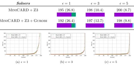
Figure 2 shows some of the results of our experiments. Each column shows the number of solved instances out of the 200 selected instances and the average runtime in seconds. The bar chart under certain cells shows the distribution of different solvers providing the results. The bottom charts present the results in a more detailed way, where the distribution of runtimes suggests that our solver can solve ca. 85–95% of the instances in less than 30 seconds.
Solvers 𝜖= 1 𝜖= 3 𝜖= 5
MiniCARD+Z3 195 (26.8) 198 (10.4) 200 (8.7) MiniCARD+Z3+Gurobi 192 (26.4) 197 (12.7) 198 (9.8)
(a)𝜖= 1 (b)𝜖= 3 (c)𝜖= 5
Figure 2. Results on checking adversarial robustness of 4-Block BNN on MNIST dataset, for different maximum perturbation val- ues 𝜖. Colors represent the ratio of solved instances by different solvers: purple forMiniCARD, green forZ3, blue forGurobi.
As the figure shows, our solver produced the best results when running
MiniCARD as a SAT solver and Z3 as an SMT solver in parallel. Since, in our preliminary experiments,Gurobihad showed promising performance, we also ran experiments withGurobi parallel toMiniCARDandZ3. Of course, we also tried different combinations of solvers in our experiments, but we found the ones in the table the most promising.
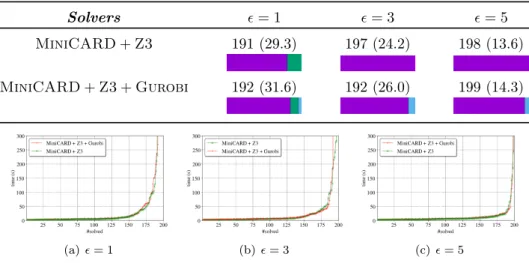
In order to investigate how our solver scales for larger BNNs, we constructed another BNN with 5 internal blocks containing Lin layers of size 300, 200, 150, 100 and 100, respectively, and trained it on the MNIST dataset. The accuracy of the resulting network is 94%. Figure 3 shows the results of our corresponding experiments.
Solvers 𝜖= 1 𝜖= 3 𝜖= 5
MiniCARD+Z3 191 (29.3) 197 (24.2) 198 (13.6) MiniCARD+Z3+Gurobi 192 (31.6) 192 (26.0) 199 (14.3)
(a)𝜖= 1 (b)𝜖= 3 (c)𝜖= 5
Figure 3. Results on checking adversarial robustness of 5-Block BNN on MNIST dataset.
6.2. Verifying network equivalence
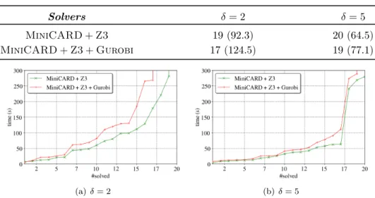
In the second set of experiments, we focused on the problem of checking network equivalence. From our 4-BlockBNN trained to classify MNIST images, we gen- erated 20 slightly different variants by altering a few weights in the network. For this sake, we randomly flip𝛿 >0weights in𝐴𝑚. Then, we run our solver to check if the original BNN is equivalent with an altered variant. Since the aim was to generate difficult benchmark instances, i.e., which are “almost UNSAT”, we chose small values for𝛿. Figure 4 shows the results of our corresponding experiments.
6.3. Side notes
In our solver’s source code, there exist implemented features that are not yet ac- cessible due to the lack of API features of certain Python packages. Although PySAT’s CNF encodings of Boolean cardinality constraints are accessible via our
Solvers 𝛿= 2 𝛿= 5 MiniCARD+Z3 19 (92.3) 20 (64.5) MiniCARD+Z3+Gurobi 17 (124.5) 19 (77.1)
(a)𝛿= 2 (b)𝛿= 5
Figure 4. Results on checking network equivalence, for different𝛿 values.
solver’s command-line argument --card-enc, equivalences (4.1) cannot directly be dealt with PySATsince the output variable of a CNF encoding cannot be ac- cessed throughPySAT’s API. For instance, we would need to access the Boolean variable 𝑣𝑛,𝑐 when using sequential counter encoding as described in Section 4.1.
Therefore, in our solver’s current version, each equivalence (4.1) is first encoded into a pair of Boolean cardinality constraints as described in Section 4.3, and the resulting cardinality constraints are then encoded into CNF. Note that encoding equivalences (4.1) directly into Boolean logic would result in more easy-to-solve instances, oncePySATallows. In the latter case, on the other hand, the encoding into CNF might dominate the runtime, since millions of variables and millions of clauses are generated even for our 4-Block BNN.
7. Conclusions
We introduced a new portfolio-style solver to verify important properties of bina- rized neural networks such as adversarial robustness and network equivalence. Our solver encodes those BNN properties, as we propose SAT, SMT, cardinality and pseudo-Boolean encodings in the paper. Our experiments demonstrated that our solver was capable of verifying adversarial robustness of medium-sized BNNs on the MNIST dataset in reasonable time and seemed to scale for larger BNNs. We also ran experiments on network equivalence with impressive results on the SAT instances.
After we submitted this paper, K. Jia and M. Rinard have recently published a paper about a framework for verifying robustness for BNNs [22]. They devel-
oped a SAT solver with native support for reified cardinality constraints and, also, proposed strategies to train BNNs such that weight matrices were sparse and car- dinality bounds low. Based on their experimental results, their solver might out- perform our solver on their benchmarks. As part of future work, we would like to run experiments with both solvers on those benchmarks.
We will try to overcome the problems that originate in using thePySATPython packages, in order to make already implemented “hidden” features accessible for users. Furthermore, we are planning to extend the palette of solvers with Google’s OR-Tools, which look promising based on our preliminary experiments.
References
[1] R. Asín,R. Nieuwenhuis,A. Oliveras,E. Rodríguez-Carbonell:Cardinality Net- works: a theoretical and empirical study, Constraints 16.2 (2011), pp. 195–221.
[2] G. Audemard, L. Simon: Lazy Clause Exchange Policy for Parallel SAT Solvers, in:
Proc. International Conference on Theory and Applications of Satisfiability Testing (SAT), vol. 8561, Lecture Notes in Computer Science, Springer, 2014, pp. 197–205.
[3] O. Bailleux,Y. Boufkhad:Efficient CNF Encoding of Boolean Cardinality Constraints, in: Proc. 9th International Conference on Principles and Practice of Constraint Programming (CP), 2003, pp. 108–122.
[4] C. Barrett,C. L. Conway,M. Deters,L. Hadarean,D. Jovanovic,T. King,A.
Reynolds,C. Tinelli:CVC4, in: Proc. Int. Conf. on Computer Aided Verification (CAV), vol. 6806, Lecture Notes in Computer Science, Springer, 2011, pp. 171–177.
[5] C. Barrett,P. Fontaine,C. Tinelli:The Satisfiability Modulo Theories Library (SMT- LIB),www.SMT-LIB.org, 2016.
[6] A. Biere:CaDiCaL, Lingeling, Plingeling, Treengeling, YalSAT Entering the SAT Compe- tition 2017, in: Proc. of SAT Competition 2017 – Solver and Benchmark Descriptions, vol. B- 2017-1, Department of Computer Science Series of Publications B, University of Helsinki, 2017, pp. 14–15.
[7] C. Cheng,G. Nührenberg,H. Ruess:Verification of Binarized Neural Networks(2017), arXiv:1710.03107.
[8] A. Cimatti,A. Griggio,B. Schaafsma,R. Sebastiani:The MathSAT5 SMT Solver, in:
Proc. Int. Conference on Tools and Algorithms for the Construction and Analysis of Systems (TACAS), ed. byN. Piterman,S. Smolka, vol. 7795, Lecture Notes in Computer Science, Springer, 2013, pp. 93–107.
[9] L. De Moura,N. Bjørner:Z3: An Efficient SMT Solver, in: Proc. Int. Conf. on Tools and Algorithms for the Construction and Analysis of Systems (TACAS), TACAS’08/ETAPS’08, Springer-Verlag, 2008, pp. 337–340.
[10] B. Dutertre:Yices 2.2, in: Proc. Int. Conf. on Computer-Aided Verification (CAV), ed.
by A. Biere,R. Bloem, vol. 8559, Lecture Notes in Computer Science, Springer, 2014, pp. 737–744.
[11] S. Dutta,S. Jha,S. Sankaranarayanan,A. Tiwari:Output Range Analysis for Deep Feedforward Neural Networks, in: NASA Formal Methods, Springer, 2018, pp. 121–138.
[12] N. Eén,N. Sörensson:An Extensible SAT-solver, in: Proc. International Conference on Theory and Applications of Satisfiability Testing (SAT), vol. 2919, Lecture Notes in Com- puter Science, Springer, 2004, pp. 502–518.
[13] R. Ehlers:Formal Verification of Piece-Wise Linear Feed-Forward Neural Networks, in:
Automated Technology for Verification and Analysis, Springer, 2017, pp. 269–286.
[14] EU Data Protection Regulation:Regulation (EU) 2016/679 of the European Parlia- ment and of the Council, 2016.
[15] M. Fischetti,J. Jo:Deep Neural Networks and Mixed Integer Linear Optimization, Con- straints 23 (3 2018), pp. 296–309,
doi:https://doi.org/10.1007/s10601-018-9285-6.
[16] M. Gario,A. Micheli:PySMT: a solver-agnostic library for fast prototyping of SMT-based algorithms, in: International Workshop on Satisfiability Modulo Theories (SMT), 2015.
[17] I. Goodfellow,Y. Bengio,A. Courville:Deep Learning, The MIT Press, 2016,isbn:
0262035618.
[18] B. Goodman, S. R. Flaxman: European Union Regulations on Algorithmic Decision- Making and a “Right to Explanation”, AI Magazine 38.3 (2017), pp. 50–57.
[19] X. Huang, M. Kwiatkowska,S. Wang, M. Wu: Safety Verification of Deep Neural Networks, in: Computer Aided Verification, Springer, 2017, pp. 3–29.
[20] I. Hubara,M. Courbariaux,D. Soudry,R. El-Yaniv,Y. Bengio:Binarized Neural Networks, in: Advances in Neural Information Processing Systems 29, Curran Associates, Inc., 2016, pp. 4107–4115.
[21] A. Ignatiev,A. Morgado,J. Marques-Silva:PySAT: A Python Toolkit for Prototyp- ing with SAT Oracles, in: Proc. International Conference on Theory and Applications of Satisfiability Testing (SAT), vol. 10929, Lecture Notes in Computer Science, Springer, 2018, pp. 428–437.
[22] K. Jia, M. Rinard: Efficient Exact Verification of Binarized Neural Networks (2020), arXiv:2005.03597 [cs.AI].
[23] G. Katz,C. W. Barrett,D. L. Dill,K. Julian,M. J. Kochenderfer:Reluplex: An Efficient SMT Solver for Verifying Deep Neural Networks, in: CAV, 2017, pp. 97–117, doi:https://doi.org/10.1007/978-3-319-63387-9_5.
[24] G. Kovásznai,A. Fröhlich,A. Biere:Complexity of Fixed-Size Bit-Vector Logics, Theory of Computing Systems 59 (2016), pp. 323–376,issn: 1433-0490,
doi:https://doi.org/10.1007/s00224-015-9653-1.
[25] J. Kung,D. Zhang,G. Van der Wal,S. Chai,S. Mukhopadhyay:Efficient Object Detection Using Embedded Binarized Neural Networks, Journal of Signal Processing Systems (2017), pp. 1–14.
[26] Y. LeCun, L. Bottou, Y. Bengio, P. Haffner:Gradient-Based Learning Applied to Document Recognition, Proceedings of the IEEE 86.11 (Nov. 1998), pp. 2278–2324.
[27] M. H. Liffiton,J. C. Maglalang:More Expressive Constraints for Free, in: Proc. Inter- national Conference on Theory and Applications of Satisfiability Testing (SAT), vol. 7317, Lecture Notes in Computer Science, Springer, 2012, pp. 485–486.
[28] B. McDanel,S. Teerapittayanon,H. T. Kung:Embedded Binarized Neural Networks, in: EWSN, Junction Publishing, Canada / ACM, 2017, pp. 168–173.
[29] M. M. McKerns,L. Strand,T. Sullivan,A. Fang,M. A. Aivazis:Building a frame- work for predictive science(2012), arXiv:1202.1056.
[30] A. Morgado, A. Ignatiev, J. Marques-Silva: MSCG: Robust Core-Guided MaxSAT Solving, JSAT 9 (2014), pp. 129–134.
[31] N. Narodytska,S. Kasiviswanathan,L. Ryzhyk,M. Sagiv,T. Walsh:Verifying Prop- erties of Binarized Deep Neural Networks, in: 32nd AAAI Conference on Artificial Intelli- gence, 2018, pp. 6615–6624.
[32] NIPS IML Symposium:NIPS Interpretable ML Symposium, Dec. 2017.
[33] T. Ogawa,Y. Liu,R. Hasegawa,M. Koshimura,H. Fujita:Modulo Based CNF Encod- ing of Cardinality Constraints and Its Application to MaxSAT Solvers, in: 25th International Conference on Tools with Artificial Intelligence (ICTAI), IEEE, 2013, pp. 9–17.
[34] G. Singh,T. Gehr,M. Püschel,M. T. Vechev:Boosting Robustness Certification of Neural Networks, in: 7th International Conference on Learning Representations, OpenRe- view.net, 2019.
[35] C. Sinz:Towards an Optimal CNF Encoding of Boolean Cardinality Constraints, in: Proc.
Principles and Practice of Constraint Programming (CP), Springer, 2005, pp. 827–831.
[36] V. Tjeng, K. Y. Xiao, R. Tedrake: Evaluating Robustness of Neural Networks with Mixed Integer Programming, in: 7th International Conference on Learning Representations, OpenReview.net, 2019.
[37] T. Weng,H. Zhang,H. Chen,Z. Song,C. Hsieh,L. Daniel,D. S. Boning,I. S.
Dhillon:Towards Fast Computation of Certified Robustness for ReLU Networks, in: ICML, 2018, pp. 5273–5282.