High-performance GPU computations in nonlinear dynamics: an efficient tool for new discoveries
--Manuscript Draft--
Manuscript Number: MECC-D-19-00713R1
Full Title: High-performance GPU computations in nonlinear dynamics: an efficient tool for new discoveries
Article Type: Original papers
Section/Category: General
Keywords: High-performance computing; GPU programming; non-linear dynamics; control of multi-stability; Keller-Miksis equation; impact dynamics; grazing impact
Corresponding Author: Ulrich Parlitz
Max-Planck-Institut fur Dynamik und Selbstorganisation Göttingen, GERMANY
Corresponding Author Secondary Information:
Corresponding Author's Institution: Max-Planck-Institut fur Dynamik und Selbstorganisation Corresponding Author's Secondary
Institution:
First Author: Ferenc Hegedüs
First Author Secondary Information:
Order of Authors: Ferenc Hegedüs
Peter Krähling Werner Lauterborn Robert Mettin Ulrich Parlitz Order of Authors Secondary Information:
Funding Information: Alexander von Humboldt-Stiftung Dr. Ferenc Hegedüs Magyar Tudományos Akadémia
(Janos Bolyai Research Scholarship) Dr. Ferenc Hegedüs Deutsche Forschungsgemeinschaft
(ME 1645/7-1) Dr. Robert Mettin
Emberi Eroforrások Minisztériuma
(BME FIKP-VIZ) Dr. Ferenc Hegedüs
Abstract: The main aim of this paper is to demonstrate the benefit of the application of highperformance computing techniques in the field of non-linear science through two kinds of dynamical systems as test models. It is shown that high-resolution, multi- dimensional parameter scans (in the order of millions of parameter combinations) via
Response to Reviewers: Dear Editor,
please find enclosed our revised manuscript entitled
"High-performance GPU computations in nonlinear dynamics: an efficient tool for new discoveries"
by Ferenc Hegedüs, Peter Krähling, Werner Lauterborn, Robert Mettin and Ulrich Parlitz, that we would like to resubmit for publication in Meccanica.
We thank both reviewers for their positive and constructive comments. In the revised manuscript text blocks printed in blue indicate new text while in red (and in brackets) we left obsolete text reviewer 2 referred to from the previous version of the manuscript.
This red text represents deleted text (please delete it during final production!).
With kind regards, on behalf of all co-authors, Ulrich Parlitz
Specific response:
Reviewer #1:
In this paper, the proposal of novel efficient computing method which can be widely used in the area of nonlinear dynamics and even in other branches of science, is demonstrated. The novelty of this concept consist in combining the so-called (by authors) "brute force" technique with high processing power of professional graphics cards. The efficiency of proposed computing procedure has been verified on the examples of two dynamical systems. The results of these numerical experiments shown that this technique allows one to discover of a new focal point of the grazing lines. Undoubtedly, these outcomes are important and original effects of this work.
In general the manuscript is well written. The introduction and description of the problem are clear and they can attract reader's interest. References are well-chosen and their number is sufficient to cover the recent research in the topic under
consideration. The effects of the research and conclusions of this article can be treated as interesting from scientific point of view. Concluding, in my opinion this paper can be interested for the readers of Meccanica, so I recommend it for publication in the present form
Dear Reviewer, we would like to thank you the effort put into our manuscript, for the very kind review and for the acceptance of our paper in its present form.
Reviewer #2:
The submitted manuscript is very good. I highly recommend it for publishing.
Please check the comments in the attached document.
Dear Reviewer, we would like to thank you to take your time and read/revise our manuscript. We extended the manuscript according to your suggestions. Below we summarize the changes in the manuscript marked by blue colour.
Section 3, first paragraph, second sentence:
This part of the manuscript is extended according to the Reviewer’s suggestion.
However, it has to mentioned that the GPU actually has only 2880 single precision cores and even less (960) double precision computing cores. In our case the double precision cores are relevant. Moreover, the comparison of the number of the cores is not a suitable indicator to estimate the speed-up. One has to inspect the peak
theoretical double precision performance that was 1707 GFLOPS for the GPU and 115 GFLOPS for the CPU. In this sense the 50 times faster GPU code is reasonable. The speed-up is also depending on how efficiently a code can exploit the peak performance (this is beyond the scope of the present paper). In our recent experience it highly depends on the problem itself; thus, 50 times speed-up is an estimate only for a specific problem (now highlighted in the manuscript).
Section 5, first paragraph:
"It is very unlikely that all attractors in the system will be discovered by taking into account only 10 random initial conditions (per single parameter settings). This might be practical for 2D/3D state-spaces. For high-dimensional state-spaces (4D and more) it takes much more initial conditions to discover all (or at least major) attractors."
This part of the paper is slightly extended. We did not aim to seek for all the attractors but only for the most relevant ones that are enough to draw meaningful conclusions.
Section 5, second paragraph:
"What when the transients are much shorter or longer?" and
"32 points on Poincaré section for last 32 periods?"
These issues are clarified in this paragraph, see the corresponding blue text. The number of needed transient iterations (2048) and the additional 8192 iterations were set according to some preliminary test calculations and with some safety factor. Yes, the last 32 iterations were used to obtain the Poincaré sections.
Section 5, Figure 1, and third paragraph:
"Those plots show the periodicity of the attractor with the highest period? What about the multi-stability - where are the other attractors (if they exist of course)?"
In the Figure caption and in the related text it is clarified now that in case of co- existence, the highest period is plotted.
Section 7, last paragraph:
"Those computations in Matlab with CPU are also brute-force, no? (just a lower resolution). Therefore, in my opinion authors should acknowledge also the
CPU+Matlab as brute force and refer to their work as "HPC/GPU brute fore approach"
We agree and we emphasised that the mentioned MATLAB + CPU computation is meant to be “brute force” here, see the blue text in the paragraph. However, we decided not to distinguish “brute force” technique performed on a GPU or a CPU.
Meccanica manuscript No.
(will be inserted by the editor)
High-performance GPU computations in nonlinear dynamics:
an efficient tool for new discoveries
Ferenc Heged ˝us · P´eter Kr¨ahling · Werner Lauterborn · Robert Mettin · Ulrich Parlitz
Received: date / Accepted: date
Abstract The main aim of this paper is to demonstrate the benefit of the application of high- performance computing techniques in the field of non-linear science through two kinds of dynamical systems as test models. It is shown that high-resolution, multi-dimensional pa- rameter scans (in the order of millions of parameter combinations) via an initial value prob- lem solver are an efficient tool to discover new features of dynamical systems that are hard to find by other means. The employed initial value problem solver is an in-house code written in C++ and CUDA C software environments, which can exploit the high processing power of professional graphics cards (GPUs). The first test model is the Keller–Miksis equation, a non-linear oscillator describing the dynamics of a driven single spherical gas bubble placed in an infinite domain of liquid. This equation is important in the field of cavitation and sono- chemistry. Here, the high-resolution parameter scans gave us the opportunity to lay down the basis of a non-feedback technique to control multi-stability in which direct selection of the desired attractor is possible. The second test model is related to a pressure relief valve
Ferenc Heged˝us
Department of Hydrodynamic Systems Faculty of Mechanical Engineering
Budapest University of Technology and Economics E-mail: fhegedus@hds.bme.hu
P´eter Kr¨ahling
Department of Hydrodynamic Systems Faculty of Mechanical Engineering
Budapest University of Technology and Economics Werner Lauterborn
Drittes Physikalisches Institut Georg-August-Universit¨at G¨ottingen Robert Mettin
Drittes Physikalisches Institut Georg-August-Universit¨at G¨ottingen Ulrich Parlitz
Research Group Biomedical Physics
Max Planck Institute for Dynamics and Self-Organization and Institut f¨ur Dynamik komplexer Systeme
Georg-August-Universit¨at G¨ottingen E-mail: ulrich.parlitz@ds.mpg.de
access/download;Manuscript;Meccanica_SpecialIssue_2019_
Click here to view linked References
1 2 3 4 5 6 7 8 9 10 11 12 13 14 15 16 17 18 19 20 21 22 23 24 25 26 27 28 29 30 31 32 33 34 35 36 37 38 39 40 41 42 43 44 45 46 47 48 49 50 51
that can exhibit a special kind of impact dynamics called grazing impact. A fine scan of the initial conditions revealed a second focal point of the grazing lines in the initial-condition space that was hidden in previous studies.
Keywords High-performance computing·GPU programming·Non-linear dynamics· control of multi-stability·Keller–Miksis equation·impact dynamics·grazing impact
1 Introduction
Non-linear dynamics has received a lot of attention since the discovery of the chaotic Lorenz attractor [1]. It opened Pandora’s box that led to a series of further discoveries of other phe- nomena such as, additional kinds of bifurcations [2, 3], multi-stability and its control [4–8], various routes to chaos and its control [9–13], transient chaotic behaviour [14, 15] or the characterisation of non-linear resonance phenomena [16–21], to name a few. Investigating a large number of classical low-dimensional equations, the above mentioned phenomena turned out to be universal features of non-linear systems. The corresponding emerging theo- ries still play an important role in the qualitative understanding of many real-life phenomena in a large variety of scientific fields, for instance, in climate dynamics [22], social sciences [23], neurobiology [24], fluid dynamics [25], mechanical engineering [26] or in laser physics [27].
Although the aforementioned studies are important, they are carried out usually on low-dimensional systems by performing investigations only in low-dimensional parameter spaces or in the local flow of the state space. That is, they require relatively low computa- tional resources compared to an up to date personal computer. However, in order to explore the complex bifurcation structure in parameter space with high resolution [28–32], the nec- essary computational power can increase by orders of magnitude. For instance, even in a two dimensional parameter plane — employing an initial value problem solver (IVP) with a resolution of 1000×1000 — the computational requirements are increased by three orders of magnitude compared to conventional 1D bifurcation plots with the same resolution of 1000. Not to mention if other important, “secondary” control parameters are involved or the application of several initial conditions is mandatory (e.g. to investigate multi-stability). The total number of the parameter combinations can easily blow-up to tens or even hundreds of millions; for instance, see our recent paper about control of multi-stability [4].
At first, it might seem impractical to try to solve a two-dimensional problem with high- resolution IVP computations, since many clever techniques exist (e.g. the pseudo-arclength continuation using a boundary value problem solver (BVP) [33]) that can explore the evo- lution of bifurcation points even in two dimensions fast and easily. Indeed, in this way, valuable information can be obtained about the bifurcation structures [4, 20, 34–37]. Never- theless, these techniques need an already found orbit to initiate the computation. Moreover, they are usually not capable to find a new set of co-existing solutions. Thus, the BVP compu- tations are always combined with IVP simulations, see the aformentioned references. In the present paper, we demonstrate that the application of parameter scans with quite high reso- lution using IVP solvers can be the source for new ideas and discoveries. For this purpose, computations are carried out on two quite different test models, for details see Sec. 2.
1 2 3 4 5 6 7 8 9 10 11 12 13 14 15 16 17 18 19 20 21 22 23 24 25 26 27 28 29 30 31 32 33 34 35 36 37 38 39 40 41 42 43 44 45 46 47 48 49 50 51
2 The history of the choice of the test models
The first test model is the periodically excited Keller–Miksis equation that is a second order ordinary differential equation describing the radial pulsation of a single spherical gas bubble placed in an infinite domain of liquid [38]. During the radial oscillation of the bubble, due to the external forcing, its contraction phase can be so rapid (collapse) that the tempera- ture inside can reach thousands of degrees of Kelvin inducing chemical reactions [39–41].
Therefore, this model is extensively used in the field of sonochemistry [42–51] to estimate the collapse strength and the chemical yield of a single bubble. In one of our previous papers [4], we extended the investigation to dual-frequency driving using two harmonic compo- nents in the external excitation. Therefore, the number of control parameters was increased to four: two driving amplitudes and two driving frequencies (for simplicity, the phase shift between the components was assumed to be zero). Our purpose was to investigate the effect of dual-frequency driving on the dynamics and the collapse strength of a bubble. The main strategy was to create high-resolution bi-parametric maps in the parameter plane of the am- plitudes at several fixed frequency pairs. However, during the evaluation of the results, due to the high resolution of the parameter space, special features of the bifurcation structure could be observed. They helped to reveal that with a special choice of the frequencies, spe- cific periodic orbits can be smoothly transformed into each other; for instance, a period-2 and a period-3 attractor. This observation inspired us to develop a non-feedback technique to control multi-stability, in which direct selection of the desired attractors is possible. To the best knowledge of the authors, such a technique was not proposed in the literature before.
The present study presents the procedure of the discovery of the technique via an extension of our original work [4].
The second test model (adapted from [52]) describes the dynamics of a pressure relief valve that can exhibit impact dynamics. It is a system of three first-order ordinary differential equations. Our main purpose was to test the special features of the numerical GPU code for non-smooth dynamical systems and reproduce some of the results presented in the original paper [52]. For some additional information about the code, the reader is referred to Sec. 3.
There is a special type of impact called grazing impact related to the oscillation of the valve body. It means that the valve body approaches the valve seat, makes contact with the valve seat with zero velocity and then moves away from the seat. At a specific parameter set, the sets of initial conditions from which the pressure relief valve exhibit grazing impact are called grazing lines. They have a focal point in the initial condition space, at which an impacting Shil’nikov-like orbit exist. The grazing lines are computed by means of a BVP solver in the paper of H˝os and Champneys [52], which was a cumbersome task that needed special care due to the discontinuous trajectories caused by the impact dynamics. According to the personal communication with the authors, the assembly of their MATLAB code took weeks. Comparing their grazing lines with our GPU accelerated IVP solver, the simulation time is reduced from a couple of hours to seconds. Moreover, the high-resolution scan of the initial conditions revealed a second focal point of the grazing lines that had been overlooked before.
It must be stressed, that in both cases, the original objective was to investigate the col- lapse strength of a single bubble or to reproduce some results corresponding to a pressure relief valve. The aforementioned discoveries are the “side effects” of the computations of high-resolution multi-dimensional parameter/initial condition scans.
1 2 3 4 5 6 7 8 9 10 11 12 13 14 15 16 17 18 19 20 21 22 23 24 25 26 27 28 29 30 31 32 33 34 35 36 37 38 39 40 41 42 43 44 45 46 47 48 49 50 51
3 The GPU accelerated solver: MPGOS
The usage of an IVP solver performing high-resolution parametric scans is sometimes called the “brute force” technique.(It usually has a low reputation in the sense that tuning up the number of the parameters, their resolution and the number of the initial conditions is not a difficult task.)It is easy to tune up the number of the parameters, their resolution and the number of the initial conditions; however, to writeefficientcomputer code to do the task within a reasonable time is far from obvious. It is especially true in our case, as we intend to employ the high processing power of professional graphics cards (GPUs). It is not trivial how to use their massively parallel hardware architecture and distribute the workload evenly to tens of thousands of parallel threads.
The developed program package (also used here) is called Massively-Parallel-GPU- ODE-Solver (MPGOS) written in C++ and CUDA C software environments and capable to distribute the tasks to multiple GPUs. It supports explicit solvers: the classic Runge–Kutta solver with fixed time-stepping, and the adaptive Runge–Kutta–Cash–Karp method with embedded error estimation of orders 4 and 5. During the simulations of the present study, the adaptive solver is used. Event handling is also incorporated into the program package. It is mandatory to be able to detect the impact in case of the pressure-relief-valve test model. In addition, with specialized user-defined functions, it is possible to manipulate the trajectories by the user after every successful time step or event detection during the GPU computations.
In this way, the impact law can be immediately applied upon the detection of an impact and the integration can be continued. Thus, it is not necessary to stop the integration or perform expensive memory transactions to apply the impact law via the CPU.(The code is quite effi- cient, a simulation is approximately about 50 times faster on an Nvidia GTX GeForce Titan Black card than on a four-core Intel Core i7-4790 CPU (using double precision floating point arithmetic)).The code is quite efficient, a simulation is approximately about 50 times faster on an Nvidia GTX GeForce Titan Black card (1707 GFLOPS peak performance) than on a four-core Intel Core i7-4790 CPU (115 GFLOPS peak performance) using double pre- cision floating point arithmetic. The parallelisation strategy in the GPU code follows the
“per-thread” approach; that is, to each GPU thread, a different instance of the investigated system is associated having different initial conditions or parameter sets. In the case of the CPU code, the different instances of the system were distributed amongst the CPU cores via the OpenMP application programming interface (API). A single CPU core solved a single instance of a system at a time. It must be emphasised that the proposed speed-up is an es- timation using the Keller–Miksis equation introduced in Sec. 4; the achievable factor in the reduction of the runtime can highly depend on the investigated ODE system (handling of special events like impact, or the number of the evaluation of transcendental functions or divisions).The detailed description of the code is beyond the scope of the present paper;
however, it has to be stressed that such a fast and efficient solver was the key to achieve the aforementioned discoveries. For more details, the interested reader is referred to the official website of the program package: www.gpuode.com or to its GitHub repository [53]. It is free to use under an MIT license and it has a detailed manual [54] with tutorial examples.
1 2 3 4 5 6 7 8 9 10 11 12 13 14 15 16 17 18 19 20 21 22 23 24 25 26 27 28 29 30 31 32 33 34 35 36 37 38 39 40 41 42 43 44 45 46 47 48 49 50 51
4 Mathematical model of the dual-frequency driven single bubble
The first test model is the Keller–Miksis equation [38]) describing the radial pulsation of a single spherical bubble placed in an infinite domain of liquid. The equation reads as
1− R˙
cL
RR¨+
1− R˙
3cL
3 2R˙2=
1+R˙
cL
+ R cL
d dt
(pL−p∞(t)) ρL
, (1)
whereR(t)is the time dependent bubble radius. The values of the material properties of the employed liquid (water) arecL=1497.3 m/s (sound speed) andρL=997.1 kg/m3(density).
According to the general, dual-frequency treatment, the pressure far away from the bubble, p∞(t) =P∞+PA1sin(ω1t) +PA2sin(ω2t+θ), (2) is the sum of a static ambient pressure,P∞, and periodic components with pressure ampli- tudesPA1andPA2, angular frequenciesω1andω2, and with a phase shiftθ. The connection between the pressures at the bubble interface can be written as
pG+pV =pL+2σ R +4µL
R˙
R, (3)
where the total pressure inside the bubble is the sum of the partial pressures of the non- condensable gas,pG, and the vapour,pV=3166.8 Pa at ambient temperature of 25oC. The surface tension isσ=0.072 N/m and the liquid kinematic viscosity isµL=8.902−4Pa s.
The gas inside the bubble obeys a simple polytropic relationship pG=
P∞−pV+2σ RE
RE R
3γ
, (4)
where the polytropic exponentγ=1.4 (adiabatic behaviour), the equilibrium bubble radius isRE=10µm and the static pressure isP∞=1 bar.
System (1)-(4) is written into a dimensionless form by introducing the dimensionless variables
τ=ω1
2πt, (5)
y1= R RE
, (6)
y2=R˙ 2π REω1
. (7)
The equations are rearranged in order to minimize the number of its coefficients. The final form is
˙
y1=y2, (8)
˙ y2= NKM
DKM, (9)
where
NKM= (C0+C1y2) 1
y1 C10
−C2(1+C9y2)−C31 y1−C4y2
y1− 1−C9y2
3 3
2y22
−(C5sin(2π τ) +C6sin(2πC11τ+C12)) (1+C9y2)
−y1(C7cos(2π τ) +C8cos(2πC11τ+C12)), (10) 1
2 3 4 5 6 7 8 9 10 11 12 13 14 15 16 17 18 19 20 21 22 23 24 25 26 27 28 29 30 31 32 33 34 35 36 37 38 39 40 41 42 43 44 45 46 47 48 49 50 51
and
DKM=y1−C9y1y2+C4C9. (11) For completeness and reproducibility, the coefficients are summarised below
C0= 1 ρL
P∞−pV+2σ RE
2π REω1
2
, (12)
C1=1−3γ ρLcL
P∞−pV+2σ RE
2π REω1
, (13)
C2=P∞−pV ρL
2π REω1
2
, (14)
C3= 2σ ρLRE
2π REω1
2
, (15)
C4= 4µL
ρLR2E 2π ω1
, (16)
C5=PA1
ρL
2π REω1
2
, (17)
C6=PA2
ρL
2π REω1
2
, (18)
C7=REω1PA1
ρLcL 2π
REω1
2
, (19)
C8=REω1PA2
ρLcL 2π
REω1
2
, (20)
C9=REω1
2πcL, (21)
C10=3γ, (22)
C11=ω2
ω1
, (23)
C12=θ. (24)
The angular frequenciesω1 andω2are normalized by the linear, undamped eigenfre- quency [55]
ω0= s
3γ(P∞−pV)
ρLR2E −2(3γ−1)σ
ρLR3E =340 kHz (25)
of the unexcited system that defines the relative frequencies as ωR1=ω1
ω0
, (26)
ωR2=ω2
ω0
. (27)
4.1 The global Poincar´e section
Due to the dual-frequency driving, the external forcing is not purely harmonic. In Eq. (10), the two dimensionless angular frequencies are 2πand 2πC11, hereC11=ω2/ω1=ωR2/ωR1
1 2 3 4 5 6 7 8 9 10 11 12 13 14 15 16 17 18 19 20 21 22 23 24 25 26 27 28 29 30 31 32 33 34 35 36 37 38 39 40 41 42 43 44 45 46 47 48 49 50 51
is the frequency ratio. The corresponding periods areT1=1 andT2=1/C11=ωR1/ωR2. For simplicity, the relative phase shift between the harmonic components is set toθ=C12=0.
During the computations, the main control parameters are the pressure amplitudes while the frequency combinations are kept fixed. The ratio of the employed frequency pairs are always rational; thus, the dual-frequency driving is still periodic (quasiperiodic forcing is excluded). This periodT, which is the smallest common multiple ofT1andT2can be used as the global Poincar´e section of the system. That is, the trajectories are sampled at time instancesτn=n·T(n=0,1,2, . . .).
5 The discovery of a non-feedback technique to directly control multi-stability In order to represent the dynamical properties of a bubble in a four-dimensional parameter space, our strategy is to compute high-resolution bi-parametric plots with the pressure ampli- tudesPA1andPA2as control parameters applying fixed relative frequency pairs (ωR1,ωR2).
The pressure amplitudes are varied between 0 and 5 bar with 501, uniformly distributed val- ues.(In order to explore the co-existing attractors, 10 randomly chosen initial conditions are used.)In order to explore the co-existing attractors, 10 randomly chosen initial conditions are used. In our experience, it was enough to find the most relevant attractors to draw mean- ingful conclusions.Thus, a single bi-parametric computation consists of approximately 2.5 million initial value problems. In the first part of the investigation, the relative frequencies are selected from the following set of values:
1 10,1
5,1 3,1
2,1 1,2
1,3 1,5
1and10
1 . (28)
Bi-parametric computations are performed at every possible relative frequency combination, meaning a total number of 36 frequency pairs (taking into account the symmetry property of the driving). In order to explore the subharmonic resonance region in more detail, an additional series of simulations were performed with every possible combination of the frequency values
2 1,3
1,4 1· · ·9
1. (29)
This means 22 additional high-resolution bi-parametric plots (taking into account again the symmetry property and the already computed pairs of frequencies during the first computa- tion period). Thus, the overall number of the solved initial value problems is approximately 145 millions.
(At each parameter combination, the first 2048 iterations are regarded as transients and discarded.)At each parameter combination, the first 2048 iterations are regarded as tran- sients and discarded.Then the system is integrated further by additional 8192 iterations to achieve convergence of averaged quantities like the Lyapunov exponent or the winding num- ber. One iteration means the integration of the system from 0 to the period of the excitation T, see Sec. 4.1.To avoid code complexity, the numbers of the iterations mentioned above are the same for all instances of the initial value problems being solved, and they are turned out to be enough according to our preliminary calculations. Thus, the convergence of the tran- sients and the average quantities are not monitored.Besides the aforementioned averaged quantities, the period, the maximum bubble radius expansion and the subsequent minimum bubble radius (important to calculate the collapse strength of the bubble oscillation) are also stored.(Furthermore, 32 points of the Poicar´e section are also recorded.)Furthermore, 32 points of the Poincar´e section of the last 32 iterations are also recorded.From the various 1
2 3 4 5 6 7 8 9 10 11 12 13 14 15 16 17 18 19 20 21 22 23 24 25 26 27 28 29 30 31 32 33 34 35 36 37 38 39 40 41 42 43 44 45 46 47 48 49 50 51
quantities, only the period and the points of the Poincar´e section are used in the present study.
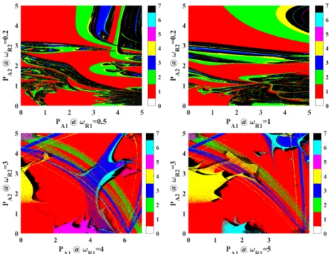
Fig. 1 Periodicity diagram of bi-parametric plots with pressure amplitudes as control parameters at different relative frequency pairs. The colour code represents the highest period (up to period-6) found at a given parameter set. Inside the black domains, there are chaotic solutions or obits having period higher than six.In the case of co-existing attractors, only the highest period is plotted.
Figure 1 shows four typical bi-parametric periodicity diagrams at different relative fre- quency combinations. The colour code represents the maximum period up to period-6 found at a given parameter set. Chaotic oscillations or orbits with periodicity higher than six oc- cupy the black regions.In the case of co-existing attractors, only the highest period is plotted.
Keep in mind that the axes in the figures represent single frequency driving since one of the pressure amplitudes is zero in these cases. The bifurcation structure in many of such dia- grams shows extreme complexity, where it is hard to find a clear regularity in the bifurcation patterns, see e.g. the upper panels of Fig. 1. However, at specific frequency combinations, bridge shaped structures appear connecting periodic segments from the vertical axis to the horizontal axis, or vice-versa. Such bifurcation structure can be clearly seen in the bottom panels of Fig. 1. Consequently, periodic orbits of single frequency driving at different rela- tive frequencies can be transformed into each other via a temporary dual-frequency driving.
The bottom-left panel of Fig. 1 is investigated in more detail in the following to give an in-depth description of the phenomenon.
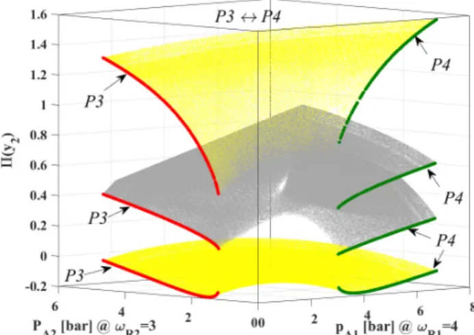
Figure 2 shows a 3D representation of the period-1 orbits (yellow and gray surfaces) corresponding to relative frequenciesωR1=4 andωR2=3, where the second component of the points of the Poincar´e sectionΠ(y2)is presented as a function of the pressure amplitudes PA1andPA2. Keep in mind that the global Poincar´e section is chosen according to the period of the dual-frequency drivingTthat is different from the period of the individual components 1
2 3 4 5 6 7 8 9 10 11 12 13 14 15 16 17 18 19 20 21 22 23 24 25 26 27 28 29 30 31 32 33 34 35 36 37 38 39 40 41 42 43 44 45 46 47 48 49 50 51
T1andT2. For the present frequency combination,T=4,T1=1 andT2=4/3≈1.333 in terms of the dimensionless timeτ. That is, the simulation defines every orbit as period-1 that repeats itself after every∆ τ=4. Therefore, for single frequency driving usingωR1=4 (T =4T1), all period-1 and period-4 orbits are treated as period-1 solutions in the dual- frequency simulations. Similarly, in case of single frequency driven system withωR2=3 (T=3T2), all period-1 and period-3 orbits are regarded as period-1 solutions if the dual- frequency Poincar´e map is applied. For an exhaustive discussion of the “period reduction”
described above, the reader is referred to our previous paper [4].
Fig. 2 The second component of the Poincar´e sectionΠ(y2)of the period-1 orbits versus the pressure- amplitude parameter plane of the dual-frequency driving.
Let us summarise the colour code in Fig. 2. The red curves represent period-3 orbits using a single frequency Poincar´e map if only the second frequency component is active (ωR2=3,PA1=0). The green curves represent period-4 orbits of single frequency driving (again using a single frequency Poincar´e map) with relative frequencyωR1=4 (PA2=0).
Finally, the yellow and grey surfaces and both the red and green curves are the second components of the Poincar´e section of period-1 orbits corresponding to the dual-frequency driving (as already discussed above). The surfaces are presented with different colours (yel- low and grey) only for the better visibility. It can be clearly seen how these surfaces make connections between the period-3 and period-4 orbits related to different relative frequency values. That is, these two kinds of orbits can be transformed into each other via a temporary dual-frequency excitation.
Although the above-described orbits are related to different relative frequency values, a special kind of control of multi-stability can be achieved in this way if the period-3 (red curves) and the period-4 (green curves) attractors have overlapping domains in the frequency-amplitude parameter plane in case of single frequency driving. However, the transformation works well even if such overlapping domains do not exist. Thus, one can still drive the system from one attractor to another regardless of their co-existence. Observe that such a control technique is a non-feedback method, but the direct selection of the de- sired attractor is also possible. Up to now, this was possible only by the feedback control techniques [6]. A thorough discussion of the advantages and the drawbacks can be found in our already mentioned previous work [4]; however, only for the transformation between 1
2 3 4 5 6 7 8 9 10 11 12 13 14 15 16 17 18 19 20 21 22 23 24 25 26 27 28 29 30 31 32 33 34 35 36 37 38 39 40 41 42 43 44 45 46 47 48 49 50 51
period-2 and period-3 orbits. Therefore, the results presented here indicate that the control technique can be generalised for other pairs of periodic orbits.
It must be emphasized that the high-resolution, multi-dimensional parameter scans have played a vital role in the discovery of the new non-feedback control technique. Since not all the bi-parametric plots show even the sign of the transformation possibility (see e.g. the top panels of Fig. 1), it is very likely that investigating only a few frequency combinations or using coarse resolutions for the pressure amplitudes, we might have missed the special bifurcation structure that led to the discovery. Moreover, as the total number of parameter combinations is of the order of a hundred million, the high-performance GPU computing was a prerequisite of this success.
6 Mathematical model of the pressure relief valve exhibiting impact dynamics The second test case describes the behaviour of a pressure relief valve that can exhibit impact dynamics. The dimensionless governing equations are adopted from [52] and are written as
˙
y1=y2, (30)
˙
y2=−κy2−(y1+δ) +y3, (31)
˙
y3=β(q−y1√
y3), (32)
wherey1andy2 are the displacement and the velocity of the valve body, respectively. The pressure relief valve is attached to a reservoir chamber in which the dimensionless pressure isy3. The fixed parameters in the system during the computations are as follows:κ=1.25 is the damping coefficient,δ=10 is the precompression parameter,β=20 is the compress- ibility parameter andq=0.3 is the dimensionless flow rate.
In Eqs. (30)-(32), the zero value of the displacement (y1=0) means that the valve body is in contact with the seat of the valve. If the velocity of the valve bodyy2has a non-zero, negative value at this point, the following impact law is applied:
y+1 =y−1 =0, (33)
y+2 =−ry−2, (34)
y+3 =y−3 (35)
That is, the velocity of the valve body is reversed by the Newtonian coefficient of restitution r=0.8 that approximates the loss of energy of the impact.
7 The discovery of a new focal point of grazing lines
During the oscillation of the valve body of a pressure relief valve, it can exhibit impact dynamics (the valve body is in contact with the valve seat) that can be categorised as follows.
The transversal impact has a non-zero velocity during the impact (y2<0); that is, it is a
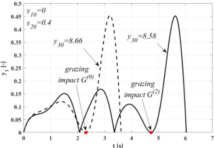
“normal” impact. Whereas, the so-called grazing impact occurs when the impact happens with a zero velocity (y2=0). In this case, the impact law has no real effect as the valve body only touches the valve seat. Figure 3 shows they1component of two trajectories that exhibit impacts (y1=0). The red dots denote the grazing impacts. The simulations are stopped at the next impact. In both cases, the initial conditions for the first two components are y10=0 andy20=0.4. The only difference is in the third initial condition:y30=8.66 and 1
2 3 4 5 6 7 8 9 10 11 12 13 14 15 16 17 18 19 20 21 22 23 24 25 26 27 28 29 30 31 32 33 34 35 36 37 38 39 40 41 42 43 44 45 46 47 48 49 50 51
y30=8.58 depicted also in the figure. The employed parameter set is summarized in Sec. 6.
The grazing impact can also be labelled (for a specific initial condition) according to how many transversal impacts there were before. Thus, in Fig. 3, the grazing impacts are denoted asG0(zero transversal impact) andG2(two transversal impacts).
Fig. 3 Time series exhibiting transversal and grazing impacts applying different initial conditions. The graz- ing impacts are marked by the red dots.
From a theoretical point of view, the generalization of the grazing impacts to they20− y30initial condition plane is an interesting problem. The first component of the initial con- dition is always set toy10=0. In this way,G(k)denotes a set of points in they20−y30initial condition plane, which leads to a grazing impact afterktransversal impacts. Throughout this paper, we shall call such a set of points as grazing lines of orderk. The first seven grazing lines computed by H˝os and Champneys [52] are shown in the bottom-right panel of Fig. 4.
Their strategy was to use a BVP solver and to employ the pseudo-arclength continuation technique to follow the path of the curves initiated from the results of an IVP solver. This formalism is quite complex, as for a single BVP, one needs to define sub-BVPs for each of thek+1 number of segments divided by the impacts. These are coupled via the impact law for the internal connections. At one side of the full-BVP, the grazing condition, while at the other side of the full-BVP, the conditiony1=0 has to be prescribed. Furthermore, the time instances of the intermediate transversal impacts need to be tracked properly as well. The main drawback of this approach is that for different values ofk, a different set of BVPs has to be set up and solved. These are the main reasons that the total computational time of a single grazing line was as high as several hours (according to personal communications with the authors). In addition, the implementation of the solver took weeks. The main outcome of the results is that the grazing lines are organized as spirals with a single focal point; and at this focal point, a Shil’nikov-like orbit exists with impacts, see again [52].
Another way to compute the grazing lines is to take an IVP solver (like our GPU ac- celerated solver), solve the system forward in time, stop the integration afterk+1 impacts and register the velocity of the endpointy2E. If this velocity is zero, the corresponding ini- tial condition lies on a grazing line of orderk denoted asG(k). With a fine resolution of the set of initial conditions in they20−y30plane, the grazing lines can be drawn easily by 1
2 3 4 5 6 7 8 9 10 11 12 13 14 15 16 17 18 19 20 21 22 23 24 25 26 27 28 29 30 31 32 33 34 35 36 37 38 39 40 41 42 43 44 45 46 47 48 49 50 51
7 8 9 10 11 12 y30
0 0.2 0.4 0.6 0.8 1
y20
G(1) G(2)
Fig. 4 Grazing lines computed by the GPU accelerated IVP solver (colour-coded panels) and the BVP solver with the pseudo-arclength continuation technique (bottom-right panel, reprinted with permission from H˝os and Champneys [52]). The pure white colour represents the zero value of velocity of the valve body of an impact (grazing impact). The pure red colour means the velocity of 1.5 m/s or higher. Between 1.5 m/s and 0 m/s, the transition is uniform in the colour code.
creating a contour plot of they2E value. Theoretically, the zero iso-lines shall represent the corresponding grazing line.
TheG(1) curve computed with our GPU-ODE solver is presented in the top-left panel of Fig. 4 via a white-red colour-coded plot. Here the integrations are stopped at the second impact (k+1=2). The resolution of the initial conditions is 1024×1024 and the total com- putation time is merely 4 s. The pure white colour represents the zero value ofy2E. The pure red colour meansy2E>1.5 m/s. Between 1.5>y2E >0, the transition is uniform in the colour code. Interestingly, the zero values always lie at a discontinuity, see the jump in the colour code labelled byG(1)in the top-left panel of Fig. 4. Accordingly, the grazing lines can be easily identified as a jump in the value ofy2E. In this sense, the task can be reduced to an edge detection problem; this is beyond the scope of the present study. The computations corresponding to theG(2)andG(5)curves are shown in the top-right and bottom-left panels of Fig. 4, respectively. In the case ofG(2), a second focal point already appears in the initial condition plane which was not observed in the BVP computations of H˝os and Champneys [52]. The two focal points are also connected with an additionalG(2)curve. Interestingly, theG(1) curve also appears as a discontinuity in they2E values; however, in either sides y2E6=0. Therefore, this curve can be seen only as a “pale” dark red-light red transition.
The reason for the non-zero velocity is that the integration is stopped at the third impact for G(2)instead of at the second one required for the detection ofG(1). Nevertheless, an edge detection algorithm can find both theG(1)andG(2)curves from a single computation with k=2. The grazing lines corresponding tok=5 are presented in the bottom-left panel in 1
2 3 4 5 6 7 8 9 10 11 12 13 14 15 16 17 18 19 20 21 22 23 24 25 26 27 28 29 30 31 32 33 34 35 36 37 38 39 40 41 42 43 44 45 46 47 48 49 50 51
Fig. 4. Similarly, as in the case ofk=2, all the previous grazing lines (k=1. . .4) are visible in the figure making it extremely complex. Thus, to detect the edges properly, a suitably fine resolution is necessary. This is not a problem in our case, as a single computation with one million initial conditions takes only a couple of seconds. Observe that in the bottom-left panel, no further focal points are discovered apart from the second one.
In summary, high-resolution scans of the initial conditions using our GPU accelarated IVP solver has revealed an additional feature (second focal point) of the grazing lines in they20−y30initial condition plane. This shows that fast “brute force” scanning is nowa- days able to discover features otherwise not visible or overlooked — here by the available BVP approach. At first sight, high-performance computation seems to be exaggerated. Even without using GPUs, the above“brute force”computations can be done within a few hours using MATLAB on a CPU. However, the main message here is that considering the usage of a “brute force” approach can lead to unexpected discoveries. Although in this specific example, high-performance computing is not really mandatory, in general, to obtain results within reasonable time for a detailed “brute force” computation, the applications of high- performance GPU (and/or CPU) clusters is usually a must.
8 Summary
In this paper, the efficacy of “brute force” technique combined with high-performance GPU computing is demonstrated through two test cases. The first model, the Keller–Miksis equa- tion, is related to the scientific topic of sonochemistry and bubble dynamics. Apart from mapping the dynamics of bubbles to obtain approximated information about their chemical activity, the bifurcation structure of the high-resolution plots led to a discovery of a new technique to control multi-stability. The second model describes the behaviour of a pressure relief valve that can exhibit non-smooth impact dynamics. Results in the literature revealed that the grazing lines — computed via a boundary value problem solver — in the initial condition plane are organized around a spiral hub. The high-resolution scans of the initial conditions using our GPU accelerated initial value problem solver led to the discovery of a new focal point of the grazing lines. In summary, “brute force” technique can play an important role in many fields of sciences, including non-linear dynamics.
In general, the prerequisite to employ high-resolution parameter scans is a fast solver.
If high computational capacities are required, a natural choice is the usage of CPU clus- ters that are available in many research institutes. The advantage of this approach is that highly optimised libraries are available for CPUs. However, GPUs have outstanding com- putational capacity/price ratio, which makes them a good alternative over CPUs. Although the parallelisation strategy for parameter scans seems to be straightforward (assign a GPU thread to each parameter combination) and libraries supporting solution of ODEs on GPUs are already available, still there can be many special issues resulting in a large performance drop.
For instance, the extremely slow CPU-GPU memory transactions need to be avoided by all costs. This can be a cumbersome task for example for systems with impact dynamics, where thousands of parallel threads (each having its own instance of the ODE with a specific parameter combination) can encounter an impact at any time. What should the programmer do if a single thread is impacting? He/she can stop the whole computation, apply the impact law on that specific thread and continue the integration process. This can be quite inefficient if the programmer has to involve CPU computations (depending on the interface and data structure of the package used), and there is always an overhead to restart the simulation 1
2 3 4 5 6 7 8 9 10 11 12 13 14 15 16 17 18 19 20 21 22 23 24 25 26 27 28 29 30 31 32 33 34 35 36 37 38 39 40 41 42 43 44 45 46 47 48 49 50 51
as well. Thus, an efficient solver has to be able to detect impact (via event handling) and manipulate the trajectory immediately “on the fly” on the GPU for each thread selectively.
There can be several other issues that may have a negative effect on code performance if GPUs are involved. Thus, tuning up the number of the parameters is easy, but a fast and efficient GPU solver usually needs a clever implementation. Such a detailed discussion is beyond the scope of the present study. Nevertheless, our GPU code is designed to efficiently address the majority of these issues. For more details, the reader is again referred to the manual of the program package [54] and to its website www.gpuode.com or to its GitHub repository [53].
1 2 3 4 5 6 7 8 9 10 11 12 13 14 15 16 17 18 19 20 21 22 23 24 25 26 27 28 29 30 31 32 33 34 35 36 37 38 39 40 41 42 43 44 45 46 47 48 49 50 51
Compliance with Ethical Standards
Funding:This study was funded by the Alexander von Humboldt Foundation (HUN 1162727 HFST-E), by the J´anos Bolyai Research Scholarship of the Hungarian Academy of Sciences, by the Deutsche Forschungsgemeinschaft (DFG) grant no. ME 1645/7-1, and by the Higher Education Excellence Program of the Ministry of Human Capacities in the frame of Water science & Disaster Prevention research area of Budapest University of Technology and Eco- nomics (BME FIKP-V´IZ).
Conflict of Interest:The authors declare that they have no conflict of interest.
References
1. E.N. Lorenz, J. Atmos. Sci.20(2), 130 (1963)
2. J. Guckenheimer, P. Holmes,Nonlinear Oscillations, Dynamical Systems, and Bifurcations of Vector Fields(Springer-Verlag, New York, 1983)
3. S.H. Strogatz,Nonlinear Dynamics and Chaos with Applications to Physics, Biology, Chemistry, and Engineering, 2nd edn. (Westview Press, Boulder, Colorado, 2014)
4. F. Heged˝us, W. Lauterborn, U. Parlitz, R. Mettin, Nonlinear Dyn.94(1), 273 (2018) 5. D. Dudkowski, A. Prasad, T. Kapitaniak, Phys. Lett. A379(40), 2591 (2015) 6. A.N. Pisarchik, U. Feudel, Phys. Rep.540(4), 167 (2014)
7. S. Wieczorek, B. Krauskopf, D. Lenstra, Opt. Commun.183(1), 215 (2000) 8. U. Feudel, C. Grebogi, B.R. Hunt, J.A. Yorke, Phys. Rev. E54, 71 (1996)
9. P. Perlikowski, M. Kapitaniak, K. Czolczynski, A. Stefanski, T. Kapitaniak, Int. J. Bifurcat. Chaos 22(12), 1250288 (2012)
10. E. Sch¨oll, H.G. Schuster,Handbook of Chaos Control(John Wiley & Sons, 2008) 11. T. Kapitaniak, J. Brindley, Chaos Soliton. Fract.9(1), 43 (1998)
12. T. Kapitaniak,Controlling Chaos(Academic Press, 1996) 13. T. Kapitaniak, Chaos Soliton. Fract.6, 237 (1995)
14. S. Sabarathinam, K. Thamilmaran, L. Borkowski, P. Perlikowski, P. Brzeski, A. Stefanski, T. Kapitaniak, Commun. Nonlinear Sci.18(11), 3098 (2013)
15. Y.C. Lai, T. T´el,Transient Chaos(Springer, New York, 2010) 16. Y. Zhang, Y. Zhang, S. Li, Ultrason. Sonochem.35, 431 (2017)
17. V. Englisch, U. Parlitz, W. Lauterborn, Phys. Rev. E92(2), 022907 (2015) 18. F. Heged˝us, C. H˝os, L. Kullmann, IMA J. Appl. Math.78(6), 1179 (2013) 19. A.J. Sojahrood, M.C. Kolios, Phys. Lett. A376(33), 2222 (2012)
20. C. Scheffczyk, U. Parlitz, T. Kurz, W. Knop, W. Lauterborn, Phys. Rev. A43(12), 6495 (1991) 21. U. Parlitz, W. Lauterborn, Z. Naturforsch. A41(4), 605 (1986)
22. S. Bathiany, M. Claussen, K. Fraedrich, Clim. Dyn.38(9), 1775 (2012) 23. K. Sneppen, N. Mitarai, Phys. Rev. Lett.109, 100602 (2012) 24. J. Braun, M. Mattia, Neuroimage52(3), 740 (2010)
25. Y.H. Shiau, Y.F. Peng, R.R. Hwang, C.K. Hu, Phys. Rev. E60, 6188 (1999) 26. C.J. H˝os, A.R. Champneys, K. Paul, M. McNeely, J. Loss Prevent. Proc.36, 1 (2015) 27. K. Pyragas, F. Lange, T. Letz, J. Parisi, A. Kittel, Phys. Rev. E61, 3721 (2000)
28. J.A. de Oliveira, L.T. Montero, D.R. da Costa, J.A. M´endez-Berm´udez, R.O. Medrano-T, E.D. Leonel, Chaos29(5), 053114 (2019)
29. F.G. Prants, P.C. Rech, Math. Comput. Simul.136, 132 (2017)
30. A.C.C. Horstmann, H.A. Albuquerque, C. Manchein, Eur. Phys. J. B90(5), 96 (2017)
31. D.R. da Costa, M. Hansen, G. Guarise, R.O. Medrano-T, E.D. Leonel, Phys. Lett. A380(18), 1610 (2016)
32. R. Rocha, R.O. Medrano-T, Int. J. Bifurcat. Chaos25(13), 1530037 (2015)
33. E.J. Doedel, B.E. Oldeman, A.R. Champneys, F. Dercole, T.F. Fairgrieve, Y.A. Kuznetsov, R. Paffen- roth, B. Sandstede, X. Wang, C. Zhang,AUTO-07P: continuation and bifurcation software for ordinary differential equations. Concordia University, Montreal, Canada (2012)
34. K. Klapcsik, R. Varga, F. Heged˝us, Nonlinear Dyn.94(4), 2373 (2018) 35. F. Heged˝us, Phys. Lett. A380(9-10), 1012 (2016)
36. U. Parlitz, V. Englisch, C. Scheffczyk, W. Lauterborn, J. Acoust. Soc. Am.88(2), 1061 (1990)
1 2 3 4 5 6 7 8 9 10 11 12 13 14 15 16 17 18 19 20 21 22 23 24 25 26 27 28 29 30 31 32 33 34 35 36 37 38 39 40 41 42 43 44 45 46 47 48 49 50 51
37. W. Knop, W. Lauterborn, J. Chem. Phys.93(6), 3950 (1990) 38. W. Lauterborn, T. Kurz, Rep. Prog. Phys.73(10), 106501 (2010) 39. L. Stricker, D. Lohse, Ultrason. Sonochem.21(1), 336 (2014)
40. D. Schanz, B. Metten, T. Kurz, W. Lauterborn, New J. Phys.14, 113019 (2012)
41. K. Yasui, T. Tuziuti, J. Lee, T. Kozuka, A. Towata, Y. Iida, J. Chem. Phys.128(18), 184705 (2008) 42. B.D. Storey, A.J. Szeri, Proc. R. Soc. Lond. A456(1999), 1685 (2000)
43. A. Brotchie, F. Grieser, M. Ashokkumar, J. Phys. Chem. C112(27), 10247 (2008) 44. R. Mettin, C. Cair´os, A. Troia, Ultrason. Sonochem.25, 24 (2015)
45. Y. Zhang, D. Billson, S. Li, Int. J. Heat Mass Transf.66, 16 (2015) 46. Y. Zhang, Y. Zhang, S. Li, Ultrason. Sonochem.29, 129 (2016)
47. J.M. Rossell´o, D. Dellavale, F.J. Bonetto, Ultrason. Sonochem.31, 610 (2016) 48. D. Dellavale, J.M. Rossell´o, Ultrason. Sonochem.51, 424 (2019)
49. H. Haghi, A.J. Sojahrood, R. Karshafian, M.C. Kolios, J. Acoust. Soc. Am.141(5), 3493 (2017) 50. H. Haghi, A.J. Sojahrood, M.C. Kolios, J. Acoust. Soc. Am.143(3), 1862 (2018)
51. H. Haghi, A.J. Sojahrood, A.C. De Leon, A. Agata Exner, M.C. Kolios, J. Acoust. Soc. Am.144(3), 1888 (2018)
52. C. H˝os, A.R. Champneys, Physica D241(22), 2068 (2012) 53. https://github.com/ferenchegedus/massively-parallel-gpu-ode-solver
54. F. Heged˝us,MPGOS: GPU accelerated integrator for large number of independent ordinary differential equation systems. Budapest University of Technology and Economics, Budapest, Hungary (2019) 55. C.E. Brennen,Cavitation and Bubble Dynamics(Oxford University Press, New York, 1995)
1 2 3 4 5 6 7 8 9 10 11 12 13 14 15 16 17 18 19 20 21 22 23 24 25 26 27 28 29 30 31 32 33 34 35 36 37 38 39 40 41 42 43 44 45 46 47 48 49 50 51
Click here to access/download
attachment to manuscript
Meccanica_SpecialIssue_2019_Revision_I_HF1.pdf
Click here to view linked References
Click here to access/download
attachment to manuscript
Meccanica_2019_ReviewerAnswer.pdf
Click here to view linked References
![Fig. 4 Grazing lines computed by the GPU accelerated IVP solver (colour-coded panels) and the BVP solver with the pseudo-arclength continuation technique (bottom-right panel, reprinted with permission from H˝os and Champneys [52])](https://thumb-eu.123doks.com/thumbv2/9dokorg/788610.36773/15.892.114.611.109.491/grazing-accelerated-arclength-continuation-technique-reprinted-permission-champneys.webp)
