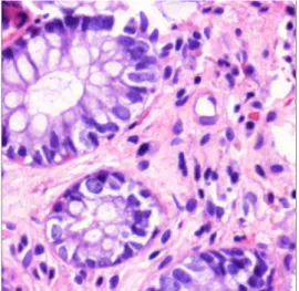
Figure 1. HE stained colon tissue
GPGPU-based Data Parallel Region Growing Algorithm for Cell Nuclei Detection
Sándor Szénási*, Zoltán Vámossy*, Miklós Kozlovszky**
* Óbuda University/John von Neumann Faculty of Informatics, Budapest, Hungary
** MTA SZTAKI/Laboratory of Parallel and Distributed Computing, Budapest, Hungary szenasi.sandor@nik.uni-obuda.hu; vamossy.zoltan@nik.uni-obuda.hu; m.kozlovszky@sztaki.hu
Abstract— Nowadays microscopic analysis of tissue samples is done more and more by using digital imagery and special immunodiagnostic software. These are typically specific applications developed for one distinct field, but some subroutines are commonly repeated, for example several applications contain steps that can detect cell nuclei in a sample image. The aim of our research is developing a new data parallel algorithm that can be implemented even in a GPGPU environment and that is capable of counting hematoxylin eosin (HE) stained cell nuclei and of identifying their exact locations and sizes (using a variation of the region growing method). Our presentation contains the detailed description of the algorithm, the peculiarity of the CUDA implementation, and the evaluation of the created application (regarding its accuracy and the decrease in the execution time).
Keywords: GPGPU, CUDA, data parallel algorithm, biomedical image processing, nuclei detection
I. INTRODUCTION
The use of digital microscopy allows diagnosis through automated quantitative and qualitative analysis of the digital images. Several procedures are based on the segmentation of the image and a lot of them need the number and the locations of the cells [2, 3]. This is usually a step of crucial importance, since normally this partial result is the basis of the further processing tasks (e.g. the higher level distinction between tissues).
There are several image processing algorithms for this purpose, but in the context of biomedical analysis there are some factors which could increase the challenge. The size of high-resolution tissue images can easily reach the order of a hundred megabytes; therefore the image processing speed plays an important factor. It is also important to realize that healthy and diseased instances of the same elements can be very dissimilar and it is hard to create an algorithm that can identify both of them.
Our work focuses on the nuclei detection on hematoxylin eosin (HE) stained colon tissue sample images (Figure 1). One of the promising alternatives is the region growing approach, which is a classical image segmentation method. The first step is to select a set of seed points which needs some suspicion about the pixels of the required region (we assume that nuclei are usually darker than their environment). In the next step it examines the neighboring pixels of the initial seed points and determines whether the pixel neighbors should be added to the region or not (by minimizing a cost function).
This process is iterated until some exit condition is met.
Region growing can correctly separate regions but the
disadvantage is the high computational cost for large images. Based on this approach, the Pannon University has developed a method [1] with reasonably good accuracy to detect cell nuclei; however, the considerably long execution time of this implementation makes the practical application quite hard.
Parallelizing the region growing algorithm aims at providing better execution times, while delivering the similar outcome produced by the sequential version. Some implementations are already published [6] but we are focusing on GPGPU applications, and most of the available solutions are unsuitable for this environment.
We need a highly data parallel algorithm and at least hundreds of threads to utilize the potential computing power of these architectures.
II. PARALLELIZING THE REGION GROWTH ALGORITHM A. Execution parameters and storage decisions
The starting point of the cell nuclei detection algorithm is a region growing procedure that – by starting off from a given seed point – aims to determine the exact size and location of the cell nucleus on that spot. The growing itself is considered to be easily parallelized, so it would be practical to implement it in a data parallel environment.
In this case the first step is determining the parameters of the execution environment (number of blocks and threads). The region growing itself consists of four consecutive steps that depend on each other: first comes the search for possible new contour expanding points, the next step is the evaluation of the available points, then comes the selection of the best valued point and the last step is the expansion of the area with the selected point.
These steps can be very well parallelized on their own, but every operation needs the output of the previous step, so we definitely need the introduction of synchronization points. This significantly reduces the count of the possible solutions, since when using a GPU, we can achieve synchronization methods with sufficient performance only within one single block. Thus, it seems practical to assign a single block to the processing of one single cell nucleus (this immediately creates a limitation for us, since the number of threads within a block is limited, in the case of the current Compute Capability 2.1 standard this value is 1024).
During the cell nucleus growing one of the most calculation- and time-consuming steps is the evaluation of the contour points, so it is advised to align the parallelization to this step. Due to the aforementioned limitation this means that during the cell nucleus search the maximum length of a contour cannot exceed 1024 pixels, but according to some preliminary research, this does not mean any problems (based on the digital images we already had, the average length of a cell nucleus contour was 125 pixels, while the longest contour was 436 pixels long).
Apart from the constant parameters, the cell nucleus searcher method itself requires a coordinate that will be the location of the starter seed point. Since multiple blocks can search for multiple nuclei at the same time, it is possible to pass on multiple seed points in the global memory of the GPU, and then start the kernel using the configuration according to these points (block settings:
single dimension, its size is the same as the number of seed points; thread settings: single dimension, its size is the maximal contour length).
Naturally, in addition to these, several other parameters must be taken into account during the execution (original and variously pre-processed images, search parameters, stop conditions); however, these do not change between the different kernel executions, so these can be kept constantly in the GPU global memory.
In addition to the parameters, the kernel utilizes several additional extra variables; these are used to store the history of the region growing (location of new points, order of insertion) and to store several other auxiliary data for the evaluation (intensity differences) and for the expansion (the points of the current region contour) as well. Most of these are not required as separate instances for every thread, so these can be practically stored in the shared memory of the GPU. The utilization of this high- speed storage significantly decreases the running time of the kernel; however, it means another important limitation for the size of the detected cell nuclei: with Compute Capability 2.1, the size of the shared memory is 48KB for every multiprocessors, and we have to take into consideration that one multiprocessor can execute more than one blocks at the same time, so this memory must be enough for all the contour data for all the blocks (and for some auxiliary data as well where it also seems practical to use this storage).
B. Region growing iteration
The region growing itself iterates three consecutive steps until one of the stop conditions is met:
1. It examines the possible directions in which the contour can be expanded. The full four-
neighborhood inspection is evidently only required around the lastly accepted contour point (when starting the kernel, this means the starting seed point). Since the examinations of the neighboring points do not depend on each other, this can be parallelized as well, the first four threads of a block examine the different neighbors, whether they are suitable points for further expansion or not (they are suitable, if they are not part of the current contour or region, or the region of another already detected cell nucleus).
2. The various different contour points must be evaluated to decide in which direction the known region should be expanded. For this, the following cost function [1] must be calculated for every points:
Where:
• I(x,y): intensity of the (x,y) neighbor
• Ir: average intensity of the region
• d(.): Euclidean distance
• (x,y)r: center of the region
• i, (x,y)i: the i-th neighbor
• α: constant
The cost function is the weighted sum of two members. The first member minimizes the intensity difference; the second minimizes the distance from the center of mass in the image space. It is important to notice that Ir and (x,y)r
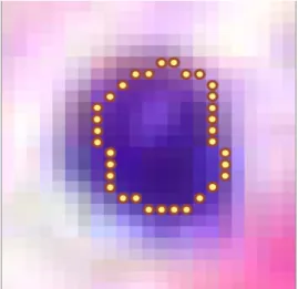
changes at the insertion of every new points, so they have to be re-calculated in every iteration for every points. This is however a typical data parallelized calculation, so it can be very well parallelized on the GPU, every thread calculate the cost of a single contour point (Figure 2).
3. The contour point with the smallest cost must be selected. The atomicMin function of the GPU can be nicely used to make the threads calculate the smallest cost, and then they can compare this with the separately calculated costs, so that the appropriate contour point can be chosen. This step in the algorithm is important, because if more than
Figure 2. GPU threads and actual contour
one thread calculates the minimal cost when evaluating a contour point, then it is totally random which of these will be selected as the winner. In contrast with the traditional CPU implementation (classical minimum selection), the GPU algorithm is not necessarily deterministic.
After every iteration, a fitness function is evaluated that reflects the intensity differences between the inner and outer contour of the region, and the circularity of the region. The process goes until the region reaches the maximum size (in pixels or in radius), and its result is the state where the maximum fitness was reached.
For the case when two cell nuclei intersect each other, another stop condition is inserted into the algorithm.
According to our experience, the overgrowing of a region into another nucleus can be detected from the intensity changes: the constantly decreasing intensity suddenly starts to increase. Due to this phenomenon, we calculate the time differential of the intensity-differences, and if the resulting function passes a given value, then we stop the region growing.
C. Post processing
After the region growing, it is practical to execute further operations on the detected regions. For example, it is worthwhile to dilate the cell nuclei to get the area’s contour as well into the resulting region. In addition to that, we should execute a fill operation too, since the resulting region can have several holes in it.
This post processing can be easily done using the classical convolution methods (erosion, dilatation). These methods can be very well implemented in data parallel environments, so this is solvable using the GPU as well [4]. The only difficulty is that these operations should not be implemented into separate kernels, because we have to use these operations very often, and the relatively high cost of starting a new kernel would significantly lower the resulting performance. Because of this, the post processing operations were implemented in the region growing kernel, which raises the limitation that the convolution operators had to be executed with the same execution parameters (one block and the biggest possible number of threads inside). It is not necessarily good for these tasks, so the theoretically possible best performance for these operators might not be reached.
After the post processing, the next step is a final evaluation based on the area of the region, on its shape (circularity), on its intensity, and on the difference between the intensity of its inner and outer contour. This is a more simple choice than the previous ones, but due to the minimization of the memory transfer, this simple evaluation is done on the GPU as well. The first thread of every block performs this evaluation, and the result is placed in the appropriate element (marked by the block index) of the resulting array. The result includes whether the cell nucleus detection was successful or not, and if yes, then the detailed data about the nucleus is included as well. After all the blocks are finished, then this array is given back to the CPU (using memory transfer), and the further processing is done there.
III. PARALLELIZING SEED SEARCH
When looking at the execution time of the whole algorithm, the search for the seed points is almost
negligible compared to the time of the region growing.
Still, it can be reasonable to implement this feature on the GPU, since the different region growing results (the point coordinates for the previously found regions) are required for the search for next seed point, so for every search these data should be transferred from the GPU memory into the CPU memory; and this would considerably worsen the execution time.
The search for seed points is a nicely parallelizable task as well, since our aim is to find the point with the highest intensity that complies with some rules (it cannot be inside a previously found region, etc). When running a sequential algorithm on the CPU, this means a single point, but in case of the GPU, this can result in multiple points, because it is possible to execute multiple cell nucleus searches in multiple blocks. In the latter case, the adjacent seed points can cause problems, since the parallelized search of those can result in overlapping cell nuclei, which would require a lot of computational time to administer. Luckily enough, we know what the maximum radius of a cell nucleus can be in an image with a given zoom; so we can presume that the searches started from two seed points (that are at least four times further apart than this known distance) can be considered as independent searches; so they can be launched in a parallelized way (Figure 3).
For this, we need a slightly more complex searching algorithm that returns with a given number of points that are in the appropriate distance from each other:
1. The points that matches the starting condition and that have the biggest intensity must be collected into an Swaiting set (since we only store the intensity on 8 bits, it is likely that there will be more that one points).
2. One element is selected from the Swaiting set, and it is moved to the Sconfirmed set.
3. In the Swaiting set, we examine the next element: we check if any of the elements from the set Sconfirmed
collide with the parallelized processing of this element (they collide, if the distance of the two points is below the critical threshold). If there is no collision, then this element is moved into the Sconfirmed as well, otherwise it stays where it is. We repeat step 3 until we run out of elements in the Swaiting set, or we find no more suitable points, or the Sconfirmed set is full (its size is the same as the number of the parallelized region growing runs we want to execute simultaneously).
Figure 3. Independent regions
4. We launch the region growing kernel using the seed points that are in the Sconfirmed set.
5. After the execution of the kernel, we store the results, we delete the contents of the Sconfirmed set, and the elements from the Swaiting set that no longer match the starting criteria.
6. If there are still elements left in the Swaiting set, we continue with step 2. If it is empty, we continue the processing with step 1.
When using this algorithm on large images, the number of possible seed points is pretty high, so it would be practical to use the GPU capabilities here as well. The algorithm uses steps that clearly depend on each other, so we can once again achieve the appropriate synchronization possibilities only when executing the calculations inside one block, for the same reasons that were described above. This limits the number of threads, so for example in the first step, every thread must iteratively inspect more than one points whether their intensity is good or not. If good points are found, then those have to be placed into the Swaiting set using atomic operations.
Since the Swaiting set probably contains many elements, it would be advised to use the data parallelized architecture in the following steps as well, which means the traditional operations have to be re-considered. The potential seed points are treated by separate threads and since the number of points is higher than the number of threads, one thread must handle more than one points, and the selection of coordinates is done in multiple steps. Every seed point is extended with a status flag, the initial status is waiting.
In the first step every thread checks if the seed points it wants to use are still usable or not (for example it is possible that during one of the previous nucleus growths the given point became occupied). The unusable points are changed into the rejected status, the others start competing with each other.
After this, every thread checks if the given seed point can be moved into the Sconfirmed set or not. If yes, then one of them (the exact one is determined by competition) moves the examined point into the Sconfirmed set, and sets the status of the seed point to processable. This iteration is continued until the thread runs out of seed points, or the required amount of points is gathered for the starting of the efficient region growing.
After the aforementioned loop ends, the first thread will load the processable seed points into the Qprocessing queue, from where the region growing will be able to load the coordinates; and then the region growing itself is started.
Since the kernels for the seed search and for the region growing require significantly different parameters (number of blocks and threads), these are implemented in two consecutive kernels.
IV. ANALYSIS OF THE ALGORITHM A. Correctness analysis
The examination of the algorithm was helped by the fact that we already have a working, CPU-based solution that was designed for similar purposes. Since the system operates with quite a lot parameters (size limits, intensity limits, various weighting factors), it is indeed convenient for the practical use to implement a different solution that gives the same output for same input data; this way the
already redeemed configuration parameters can be easily used, and there is no need for further experimentation and proving.
The implemented GPU algorithm (using certain settings) should be able to give exactly the same results as the CPU implementation (we did use this feature during our tests); but due to some characteristics of the GPU we can expect a slightly more accurate information there than with the CPU: the GPU can typically execute faster operations using floating point numbers, so we used the more accurate floating point version for all the numbers, even for those where (for the sake of optimization) integers were used in the CPU version.
When comparing to the CPU implementation, we have another advantage: in the case of the GPU implementation (much alike other GPU algorithms) the typical limitation factor for the performance is not the number of calculations, but rather the number of memory operations.
So even if we should use certain simplifications with the CPU (e.g. we should not re-calculate the fitness function for all the points if the centre of mass and the intensity of the nucleus has not changed much), we do not need those simplifications with the GPU: these calculations can be easily done in every iteration using the enormous computational capacity that the GPU offers. Without the simplifications, the result we obtain is slightly more accurate.
Due to the large size of the images, the evaluation was done using an application that compared the regions found by the CPU and the GPU implementations. This tester application tried to pair up the regions found by the two implementations, and it compared the paired regions based on the pixels, and as a result it classified the output based on the (number of different pixels) / (sum size of regions) value.
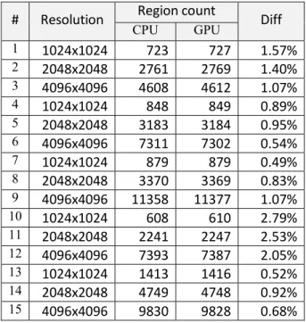
Altogether we examined 41 samples using this method (with sizes 1024x1024, 2048x2048 and 4096x4096; and with mixed contents such as intact tissues, diseased tissues and badly focused images). Based on this examination, the average difference is 1.30%. The first 15 records can be found in Table 1.
# Resolution Region count
Diff
CPU GPU
1
1024x1024 723 727 1.57%
2
2048x2048 2761 2769 1.40%
3
4096x4096 4608 4612 1.07%
4
1024x1024 848 849 0.89%
5
2048x2048 3183 3184 0.95%
6
4096x4096 7311 7302 0.54%
7
1024x1024 879 879 0.49%
8
2048x2048 3370 3369 0.83%
9
4096x4096 11358 11377 1.07%
10
1024x1024 608 610 2.79%
11
2048x2048 2241 2247 2.53%
12
4096x4096 7393 7387 2.05%
13
1024x1024 1413 1416 0.52%
14
2048x2048 4749 4748 0.92%
15
4096x4096 9830 9828 0.68%
Table 1. CPU/GPU results comparison
It is noteworthy that a difference in the results not necessarily mean that one of the algorithms are faulty, it simply means that the task has more than one solutions (depending on the order the seed points are processed), and the different executions found different solution with the same fitness value.
B. Execution time by block size
Due to the design principle of the GPU, the performance of a single execution unit is far behind the performance of a single CPU core; the key point of the final performance is utilizing the big number of the available execution units. The algorithm of course supports this, since for every contour point we dedicate a thread; however, determining the exact number of threads is a critical question: to maximally utilize the parallel execution, we should start the maximum possible number of threads, but due to the characteristics of the GPU hardware, if one block requires too many threads (too many resources), then this circumstance decreases the number of blocks that can be executed by a single multiprocessor.
For this reason, it is advised to examine how big regions are the best to maximally utilize the performance of the GPU. On one hand, this gives us the possibility to fine-tune the algorithm (we can define the number of threads for the search of one cell nucleus according to this feature), and it gives us a good recommendation to know how big the input image should be scaled to.
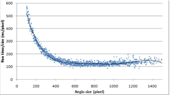
We ran tests and by collecting data from several tests we measured how fast the GPU could process different regions of different sizes (altogether we tested 127000 regions, we compared the execution times). The bigger regions of course mean bigger execution time, so for the sake of testing it is better to use a relative measurement unit, so that we can compare speed changes between different region sizes. The unit we used was that we calculated that relatively how long it took to process one pixel within a region. It is clearly visible (Figure 4) that when using small regions, this value is considerably high, and by increasing the region size, this value decreases rapidly. Using the tested settings, this cost function reaches its minimum value at around 600 pixels, after that point it does not decrease significantly. Compared to the worst (~600ms/pixel) result, the ~120ms/pixel value means a significantly, four times faster operation. So to use the performance of the GPU in the most efficient way, it is practical to scale the input image to have the cell nuclei with about this size (regions bigger than 1200 pixels are quite rare anyways, so because of the big
deviation, the slight increase we can see in this interval is not relevant).
Also, to evaluate the performance, it is important to compare the performance of the GPU implementation with the performance of the CPU implementation. This is shown in Figure 5.
As it was expected, with the CPU implementation, the execution time became a little smaller if we used smaller region sizes, and although the graph is a little less steeply, the values do decrease as we increase the region sizes.
Interestingly enough, the CPU (even thought it executes a significantly different algorithm) reaches the ideal speed at the same region size value where the GPU. Here (around 600 pixels and above) the GPU can start enough threads so that their cumulative computational power approaches the computational power of the CPU.
However, it is clearly visible on the figures that the GPU can only approach, but it cannot reach the computational power of the CPU (GPU ~600ms/pixel - CPU
~500ms/pixel; GPU ~120ms/pixel - CPU ~100ms/pixel).
C. Execution time by number of blocks
At first sight, these results can cause disappointment, because despite the massive peak performance of the GPU, due the characteristics of the algorithm (due the synchronizations and the auxiliary operations) the performance of the CPU cannot be reached. But the aforementioned values only show the examination of the increase in the region size, which affects (in the current implementation) only the operation of the single blocks. If the input is suitable (there are enough distant-placed starting points with similar intensities) then it is possible to start several blocks (thus, several region growth) at the same time.
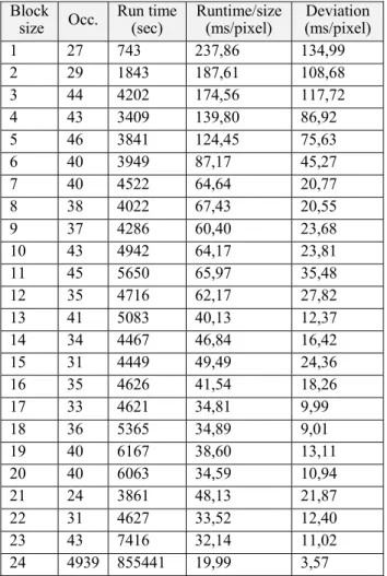
For these reasons, we started a new measurement, but now we did not measure the performance based on the region size, rather based on the number of concurrent region operations the GPU handled (for results, see Table 2)
We tested the algorithm on significantly large images, so most times (4939 times) the GPU could utilize the maximum parallelism (which is, at the current configuration, 24 blocks at the same time, but this can be changed easily). The smaller block sizes are (on one hand) quite rare, on the other hand they mostly occur in special cases (processing of remainder areas, mostly small regions). For this reason, the deviation of the measured times is relatively high, and the times shown here do not necessary reflect the maximum performance (that is why the execution times shown here differ from the previously found optimum time of single block execution).
Figure 5. Region growth execution time on CPU
Figure 4. Region growth execution time on GPU
It is visible (Figure 6) that if we managed to increase the number of blocks as well, then the relative execution time of one pixel started to drop significantly. This drop is visible until the parallel execution of the 17th block, here the GPU reached its peak performance, the execution of further blocks do not affect the measured times that much.
The 20ms/pixel value that we can see with 24 blocks is far better than even the best results of the CPU (if we look at only the numbers, we might consider a larger block size, but this will not change the results, because the value for the largest block size will always be smaller than the value before the preceding ones, since the ideally located large regions usually processed with this block size).
To measure the execution time, we always used the QueryPerformanceCounter function, the accuracy of this timer is approximately 0.366 µs, starting and stopping the timer means approximately a 3 µs error during the measurement. By looking at the results, it can be stated that these errors are negligible. The above presented results always show the average of five independent measurements, after which the measurement error seemed sufficiently low (variance coefficient < 0.002%) to safely draw a conclusion. Furthermore, in the GPU measurements, we excluded the time of the first launch of the kernel (independent from the number of blocks in the first kernel), because it is possible that during the first launch the GPU (or the GPU driver) might experience additional time costs that may distort the results.
D. Execution time by image resolution
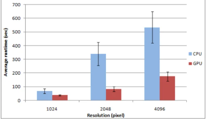
Thought the aforementioned results are also important for further optimization, for the practical use, the most important question is the analysis of the required time to process a whole image. For this, we executed the CPU and the GPU implementation with different sized images with different contents.
The input of the complete execution time test were 13 slides in three different resolutions (1024x1024 pixels, 2048x2048 pixels and 4096x4096 pixels).
Figure 7 shows the execution time in the case of the largest images.
The GPU implementation is always faster than the CPU implementation: minimum 2 times but in some cases 8 times faster. These differences are varied and strongly depend on the image content (number of cells, ratio of empty and filled areas, etc.), therefore it is hard to forecast the prospective gain in speed.
Resolution Impl. Average execution time
(sec)
Std.
deviation (sec) 10242
CPU
68.5 17.3
GPU
38.2 5.3
55.8%
20482
CPU
339.5 84.6
GPU
83.2 18.2
24.5%
40962
CPU
533.5 116.3
GPU175.0 33.5
32.8%
Table 3. Execution time by number of blocks Figure 7. Execution time for 4096x4096 images
Figure 6. Execution time by number of blocks Block
size Occ. Run time (sec) Runtime/size
(ms/pixel) Deviation (ms/pixel)
1 27 743 237,86 134,99
2 29 1843 187,61 108,68
3 44 4202 174,56 117,72
4 43 3409 139,80 86,92
5 46 3841 124,45 75,63
6 40 3949 87,17 45,27
7 40 4522 64,64 20,77
8 38 4022 67,43 20,55
9 37 4286 60,40 23,68
10 43 4942 64,17 23,81
11 45 5650 65,97 35,48
12 35 4716 62,17 27,82
13 41 5083 40,13 12,37
14 34 4467 46,84 16,42
15 31 4449 49,49 24,36
16 35 4626 41,54 18,26
17 33 4621 34,81 9,99
18 36 5365 34,89 9,01
19 40 6167 38,60 13,11
20 40 6063 34,59 10,94
21 24 3861 48,13 21,87
22 31 4627 33,52 12,40
23 43 7416 32,14 11,02
24 4939 855441 19,99 3,57
Table 2. Execution time by number of blocks
The same benchmarks have been performed on all available resolutions; Table 3 shows the cumulative results (execution time of the CPU and GPU implementation and the GPU/CPU time ratio). Figure 8 shows the same results in a perspicuous diagram.
As our test results affirmed, the GPU usage was able to speed up the image processing tasks significantly. It can be stated that (even thought the smaller images can be processed faster with the graphics unit as well) the real benefits of the GPU come to the front at higher resolution.
CONCLUSIONS
The main aim of the research was the development of a new algorithm to determine the number of cell nuclei along with their locations and their sizes in an HE stained tissue sample that is capable of being executed in a data parallel environment.
In the current phase of the research, the algorithm and its CUDA implementation are completed. According to our tests its positive hit rate is similar as (or in some cases, it is better than) the results of the currently available
similar solutions; the execution time is (depending on the image size) about 25–65% of the original CPU implementations. Since in the case of bigger images, the execution time of the traditional sequential algorithms can reach even 30 minutes, this is not only a technical optimization result: this approach may make an accurate, but (due to performance reasons) a so far unusable principle into a practically usable medical solution.
If the further decrease in the execution time is considered to be the main purpose of the further developments, then it is necessary to create a version of the described algorithms that support several GPUs (or even a solution that uses several GPUs and the CPU too, to perform synchronization or actual region growing tasks in the CPU as well).
REFERENCES
[1] Pannon Egyetem, “Algoritmus- és forráskódleírás a 3DHistech Kft. számára készített sejtmag-szegmentáló eljáráshoz”, 2009 [2] A. Reményi, S. Szénási, I. Bándi, Z. Vámossy, G. Valcz, P.
Bogdanov, Sz. Sergyán, M. Kozlovszky, "Parallel Biomedical Image Processing with GPGPUs in Cancer Research", LINDI 2011, Budapest, 2011 ISBN: 978-1-4577-1840-3, IEEE Catalog Number: CFP1185C-CDR, pp. 245–248
[3] L. Ficsór, V. S. Varga, A. Tagscherer. Zs. Tulassay, B. Molnár.,
"Automated classification of inflammation in colon histological sections based on digital microscopy and advanced image analysis." Cytometry, 2008. pp. 230–237.
[4] Podlozhnyuk, Victor., "Image Convolution with CUDA." s.l. : NVIDIA, 2007.
[5] A, Nagy, Z. Vámossy. “Super-Resolution for Traditional and Omnidirectional Image Sequences” Acta Polytechnica Hungarica, Vol. 6/1, Budapest Tech, 2009. pp. 117–130, ISSN 1785 8860 [6] P.N. Happ, R. S. Ferreira, C. Bentes, G. A. O. P. Costa, R. Q.
Feitosa: “Multiresolution Segmentation: A Parallel Approach For High Resolution Image Segmentation in Multicore Architectures”, GEOBIA 2010, Ghent, 2010
Figure 8. Execution time by resolution