Bayesian inference to partition determinants of community dynamics from observational time series

(1)

Community ECology 20(3): 238-251, 2019 1585-8553 © AkAdémiAi kiAdó, BudApest

dOi: 10.1556/168.2019.20.3.4

1. Introduction

Fluctuations in population abundance or biomass within ecological communities result from a complex interplay of abiotic and biotic factors combined with demographic stochasticity or ecological drift (Lande et al. 2003, Loreau and de Mazancourt 2008, Mutshinda 2009, 2010). The abiotic factors involve environmental forcing mediated by changing physical conditions (e.g., temperature) and/or fluctuations in the availability of non-living resources affecting the growth, reproduction and maintenance of organisms. The biotic forc- and maintenance of organisms. The biotic forc-maintenance of organisms. The biotic forc- biotic forc- es include density-dependent feedbacks and species-species interactions within and across trophic levels. Negative density dependent regulation is a pervasive feature of population growth processes (Nicholson 1933, Cooper 2003, Brook and Bradshaw 2006), and may result from competition for limiting resources among conspecifics (intra-specific competition) or from other mechanisms operating in a density-dependent fashion such as predation and diseases. �emographic sto-�emographic sto-

chasticity refers to the variability in population growth resulting from randomness in outcomes of demographic events (births, deaths, dispersal) across individuals in a finite population (Lande et al. 2003).

Community dynamics models that integrate these various sources of variability enable better understanding of the caus-understanding of the caus- es of shifts in community structure and allow sensible predic-and allow sensible predic- tions of community responses to environmental fluctuations.

So far, models concerned with ecological responses to envi-odels concerned with ecological responses to environmental changes have mostly focused on abiotic forcing with less regard to biotic interactions (Gilman et al. 2010).

However, there is an emerging consensus among ecologists on the major role of biotic interactions in structuring ecological communities and modulating population responses to climate change (e.g., �avis et al. 1998a,b, Araujo and Luoto 2007, Heikkinen et al. 2007, Gilman et al. 2010, Götzenberger et al. 2012). �et, the modelling and �uantifi cation of biotic in-). �et, the modelling and �uantifi cation of biotic in-. �et, the modelling and �uantifi cation of biotic in- �uantification of biotic interactions is challenging, particularly for species-rich systems such as microbial or planktonic assemblages due to the huge

Bayesian inference to partition determinants of community dynamics from observational time series

C. M. Mutshinda

^1,4

, Z. V. Finkel

²

, C. E. Widdicombe

³

and A. J. Irwin

¹

1Department of Mathematics and Statistics, Dalhousie University, Halifax, NS, Canada

2Department of Oceanography, Dalhousie University, Halifax, NS, Canada

3Plymouth Marine Laboratory, Prospect Place, Plymouth, PL1 3DH, UK

4Corresponding author, Email: crispin.mutshinda@dal.ca

Keywords: Bayesian inference; Biotic interactions; Community dynamics; Environmental forcing; Markov chain Monte Carlo;

Spike-and-slab prior.

Abstract: Ecological communities are shaped by a complex interplay between abiotic forcing, biotic regulation and demographic stochasticity. However, community dynamics modelers tend to focus on abiotic forcing overlooking biotic interac- biotic interactions, due to notorious challenges involved in modeling and �uantifying inter-specific interactions, particularly for species-rich systems such as planktonic assemblages. Nevertheless, inclusive models with regard to the full range of plausible drivers are essential to characterizing and predicting community response to environmental changes. Here we develop a Bayesian model for identifying, from in-situ time series, the biotic, abiotic and stochastic factors underlying the dynamics of species-rich com- and stochastic factors underlying the dynamics of species-rich com- factors underlying the dynamics of species-rich communities, focusing on the joint biomass dynamics of biologically meaningful groups. We parameterize a multivariate model of population co-variation with an explicit account for demographic stochasticity, density-dependent feedbacks, pairwise interactions, and abiotic stress mediated by changing environmental conditions and resource availability, and work out explicit formulae for partitioning the temporal variance of each group in its biotic, abiotic and stochastic components. We illustrate the methodology by analyzing the joint biomass dynamics of four major phytoplankton functional types namely, diatoms, dinofl a-diatoms, dinoflagellates, coccolithophores and phytoflagellates at Station L4 in the Western English Channel using weekly biomass records and coincident measurements of environmental covariates describing water conditions and potentially limiting resources. Abiotic and biotic factors explain comparable amounts of temporal variance in log-biomass growth across functional types. Our results demonstrate that effective modelling of resource limitation and inter-specific interactions is critical for �uantifying the relative importance of abiotic and biotic factors.

Abbreviations: AR model–Autoregressive model; BUGS–Bayesian inference Using Gibbs Sampling; LASSO–Least Absolute Shrinkage and Selection Operator; MCMC–Markov Chain Monte Carlo; PSU–Practical Salinity Unit; VAR model–Vector Autoregressive model.

(2)

Bayesian inference on community dynamics 239 number of potential interactions between species (Ovaskainen

et al. 2017), raising the curse of dimensionality as the number of pairwise interactions increases exponentially with the number of populations under consideration. As a result, commu-community dynamics models, typically vector autoregressive models (VAR) models models, are often restricted to a few popula- models, are often restricted to a few popula- are often restricted to a few populations. VAR models, which extend univariate autoregressive (AR) models to multivariate time series, provide a flexible framework for analyzing the joint dynamics of co-occurring populations and evaluating, from observational time series, the biotic, abiotic, and stochastic factors drivers of population dynamics and community structure (Ives et al. 2003, Mutshinda et al. 2009, 2011, Hampton et al. 2013). A VAR model of order p, denoted as treats each endogenous variable as a linear function of its own p lags and the lags of all other endogenous variables in the system. VAR models of any order p > 1 can be rewritten in the form, which is more convenient for analytical operations. Underlying autoregressive models of order 1 is the assumption that the future is independent of the past given the present, known as the Markov property.

VAR models of species-rich assemblages typically require some kind of complexity reduction to overcome the curse of dimensionality resulting from the huge number of parameters, particularly the inter-specific interactions coefficients (e.g., Ovaskainen et al. 2010, Pollock et al. 2014, Clark et al. 2018). Kissling et al. (2012) review complexity reduction techniques for modelling biotic interactions in species-rich assemblages, separating them into statistical and ecological methods. Statistical methods for complexity reduction hinge essentially on the assumption that weak interactions prevail in natural communities (Mutshinda et al. 2009, 2011) and accordingly, attempt to produce a sparse interaction matrix by resorting to sparsity-inducing methods. In the Bayesian framework (McCarthy 2007, Gelman et al. 2013), sparsity- inducing methods can be categorized into indicator-based variable selection methods and regularization or shrinkage techniques. Indicator-based variable selection techniques (e.g., George and McCulloch 1993) achieve sparsity by ex-George and McCulloch 1993) achieve sparsity by ex-) achieve sparsity by excluding the redundant predictors from the model. On the other hand, regularization methods (e.g., Park and Casella. 2008, Mutshinda and Sillanpää 2010, 2011, 2012) keep all potential predictors in the model, but impose a penalty constraining the magnitudes of their coefficients to shrink towards zero, caus- ing the effects of redundant predictors to be zero or nearly so and virtually excluding such predictors from the model.

The most popular regularization methods are the LASSO (Tibshirani 1996) and ridge regression (Hoerl and Kennard 1970) which constrain the L₁ and L₂ norm of the coefficient vectors, respectively. Because of its ability to set some of the coefficients exactly to zero, the LASSO is increasingly popular as a variable selection tool. We refer to O’Hara and Sillanpää (2009) for an extensive review of Bayesian variable selection methods. The rationale of ecological methods for complexity reduction is to aggregate the plethora of species under consideration in a few biologically meaningful groups such as organismal taxonomic units or functional types, and focus on group-level data. This is pragmatic since it is much easier to deal with a handful of groups than many individual

species. In addition, species-level data are usually fraught with missing values. The aggregation of species into a few biologically meaningful groups may also be required by the question being addressed. For instance, when designing models for predicting phytoplankton biomass or characterizing traits, it is useful to aggregate the host of species into functional types based on distinctive ecological functionality or chemical roles, which are sensible proxies for ecological and biogeochemical functions (Le Quéré et al. 2005, Irwin and Finkel 2018).

In this paper, we develop a Bayesian model for evaluat-a Bayesian model for evaluating, from long-term monitoring data, the factors and mechanisms underlying the structure and dynamics of species-rich communities, focusing on the joint biomass dynamics of biologically meaningful groups. We parameterize a multi- parameterize a multivariate model of group biomass co-variation integrating demographic stochasticity, density-dependent effects, pairwise interactions, and abiotic stress mediated by changing environmental conditions and limiting resources. We devise formulae for partitioning the temporal variance in log-biomass growth of each group in its biotic, abiotic and stochastic components. We illustrate the method by analyzing the joint biomass dynamics of four major phytoplankton functional types namely, diatoms, dinofl agellates, coccolithophores and phy-diatoms, dinoflagellates, coccolithophores and phytoflagellates using long-term data recorded at Station L4 in the Western English Channel as part of the Western Channel Observatory oceanographic time series (Widdicombe et al.

2010a,b). The data involve weekly biomass concentrations of the four functional types and coincident measurements of five environmental covariates. Two of the environmental covariates (temperature and salinity) describe environmental conditions whereas the other three (irradiance, nitrogen, and silicate) represent potentially and limiting resources.

2. Materials and methods

In the sequel, boldface lower-case letters and boldface capital letters represent vectors and matrices, respectively.

2.1. Model specification

We describe the biomass dynamics of each taxonomic group by a stochastic Gompertz model extended to incorporate pairwise interactions and external forcing mediated by changing environmental conditions (temperature or salinity) and potentially limiting abiotic resources (irradiance, nitrogen, and silicate). The separation of environmental covariates into environmental conditions and limiting resources is important since they enter the model differently. Henceforth, we refer to the covariates describing environmental conditions as environmental conditions. Let Y_i,t and X_q,t denote respectively, the biomass of the ith taxonomic group (i = 1,..., n) and the Z-score of the qth environmental condition at time t (t ≥ 2). We assume that

(1)

5

group (𝑖= 1, … ,𝑛) and the Z-score of the qth environmental condition at time t (𝑡 ≥2). We 128

assume that 129

𝑌�,�=𝑌�,�� exp� 𝑟�,��1 +� 𝛼��

𝑘� ln(𝑌�,��)

�

�� +� 𝑋�,�

�

�� 𝛽�,�+𝜀�,�� (1)

where 𝑟�,�> 0 denotes the density-independent growth rate of the ith group from time 𝑡 −1 to 𝑡 130

at average environmental conditions, 𝛽_�,� represents the effect of the qth environmental condition 131

(temperature or salinity) on the ith group, and 𝜀_�,� is a zero-mean random disturbance affecting 132

the biomass dynamics of the ith group at 𝑡. The interaction coefficient 𝛼_�,� (𝑖 ≠ 𝑗) represents the 133

effect of the jth group’s biomass on the growth rate of the ith group, relative to the effect of the 134

ith group’s biomass on its own growth rate. The scaling factor 𝑘_�> 0 is the carrying capacity of 135

the ith group’s log-biomass. We set all intraspecific interaction coefficients 𝛼_�,� to -1 for 136

identifiability purposes. In its typical form, the Gompertz model has a minus sign in front of the 137

density-dependent term ∑ ^�_�^��

� ln(𝑌�,��)

�� appearing in the exponent of equation (1), with all 138

intraspecific interaction coefficients 𝛼�,� set to 1 (Mutshinda et al. 2009, 2011). Here we use a 139

positive sign instead so that negative and positive coefficients portray detrimental and beneficial 140

impacts respectively, hence the choice of -1 for the intraspecific coefficients. �epending on its 141

sign and magnitude, the inter-specific interaction can be detrimental to both participants 142

(competition), detrimental to one and beneficial to the other (exploitation or antagonism), 143

detrimental to one without cost or benefit to the other (amensalism), of no effect to either 144

participant (neutralism), or beneficial to at least one of the participants with no harm to either 145

(facilitation). Facilitation can take the form of mutualism if both participants benefit or 146

commensalism when it only benefits one of them (Stachowicz 2001).

147

For purposes of estimating the model parameters, it is convenient to work on a 148

logarithmic scale. Re-writing (1) on the natural logarithmic scale with 𝑦_�,� representing the 149

natural logarithm of 𝑌_�,� yields 150

𝑦�,�=𝑦�,��+𝑟�,��1 +� 𝛼�,�

𝑘� 𝑦�,��

�

�� +�^� 𝑋�,� 𝛽�,�+

�� 𝜀�,� (2)

(3)

240 Mutshinda et al.

where r_i,t> 0 denotes the density-independent growth rate of the ith group from time t–1 to t at average environmental conditions, b_i,q represents the effect of the qth environmental condition (temperature or salinity) on the ith group, and e_i,t is a zero-mean random disturbance affecting the biomass dynamics of the ith group at t. The interaction coefficient a_i,j (i ≠ j) represents the effect of the jth group’s biomass on the growth rate of the ith group, relative to the effect of the ith group’s biomass on its own growth rate. The scaling factor ki

> 0 is the carrying capacity of the ith group’s log-biomass. We set all intraspecific interaction coefficients ai,i to –1 for identifiability purposes. In its typical form, the Gompertz model has a minus sign in front of the density-dependent term

appearing in the exponent of equation (1), with all intraspecific interaction coefficients a_i,i set to 1 (Mutshinda et al. 2009, 2011). Here we use a positive sign instead so that negative and positive coefficients portray detrimental and beneficial impacts respectively, hence the choice of –1 for the intraspecific coefficients. Depending on its sign and magnitude, the inter-specific interaction can be detrimental to both participants (competition), detrimental to one and beneficial to the other (exploitation or antagonism), detrimental to one without cost or benefit to the other (amensalism), of no effect to either participant (neutralism), or beneficial to at least one of the participants with no harm to either (facilitation).

Facilitation can take the form of mutualism if both participants benefit or commensalism when it only benefits one of them (Stachowicz 2001).

For purposes of estimating the model parameters, it is convenient to work on a logarithmic scale. Re-writing (1) on the natural logarithmic scale with yi,t representing the natural logarithm of Y_i,t yields

�enoting the change (growth) yi,t – yi,t–1 in the log bio-log biomass of the ith group from time t – 1 to t by Dy_i,t, it follows from (2) by direct differentiation and re-arranging of terms that

Conse�uently, the inter-specific interaction coefficient a_i,j

�uantifies the effect of group j on the growth rate of group i, relative to the (negative) feedback ∂Dyi,t/∂yi,t–1 of the ith group’s biomass on its own growth rate from time t – 1 to t, whose magnitude is h_i,t = r_i,t|a_i,i|/k_i or simply r_i,t/k_i since |a_i,i|

= 1 by design.

In compact matrix notation, the joint dynamics model (2) for a n-group system reads

y_t = y_{t – 1} + R (1_n + Ay_{t –1}) + ß x_t + e_t (4)

where y_t = (y_i,t, ..., y_n,t)^T and x_t = (X_1,t, ..., XQ,t)^T denote respec-denote respectively the n-vector of group-level log-biomasses and the Q–

vector of Z-scores of the environmental conditions at time t, R is the n×n diagonal matrix with R(i,i) = r_i, 1_n is the n-vector of ones, A is the n×n matrix with (i,j)th entry A_i,j= ai,j/ki, ß is the n×Q matrix with ith row (bi,1, ..., bi,Q), and e_t= (e1,t, ..., en,t) is the n-vector of zero-mean random disturbances affecting the biomass dynamics of the n groups at time t. We assume that the error vectors e_t (t ≥ 2) are serially independent, but allow the contemporaneous components e_1,t, ..., e_n,t of e_t to co- vary, so that we can evaluate potential dependencies among groups that the involved covariates may not capture. More specifically, we assume that each e_t is multi-normally distributed around the n-dimensional zero vector with a potentially non-diagonal covariance matrix V_t. The residual variances (the diagonal entries of Vt) lump together the group-specific variances due to potentially important covariates that may be omitted from the model with demographic stochasticity and sampling error. �emographic stochasticity can be extracted by capitalizing on its inverse scaling with the population size or biomass. If we assume that sampling variation is negligible, then we can decompose the residual covariance matrix as V_t = D_t + C (5) where D_t is a n×n time-dependent diagonal matrix, with D_t(i,i) = d_i/Y_i,t–1 representing the demographic stochasticity affecting the biomass dynamics of the ith group from time t – 1 to t, and d_i > 0 denoting the demographic variance parameter specific to the ith group. �ue to its inverse scaling with the population size or biomass, demographic stochastic-the population size or biomass, demographic stochastic-demographic stochasticity is only relevant for small populations (e.g., Saether et al.

2000, Lande et al. 2003, Mutshinda et al. 2009, 2011). The second component of V_t is the n×n time-independent residual environmental covariance matrix C whose diagonal elements C_i,i, and off diagonal elements C_i,j (i ≠ j) represent respectively the group-specific and joint responses to un-modelled environmental factors.

Resource limitation to the growth of individual groups is not explicit in the model described by equations (1) and (2), but is potentially important. To facilitate the variance decomposition analysis, we consider two different versions of the model namely, a reduced model represented by equations (1) and (2) with r_i,t = r_i(independently of time), and a full model involving an explicit account of resource limitation. In the full model, we incorporate resource limitation by letting r_i,t = m_if_i(t), where m_i > 0 is the maximum net growth rate of the ith group from one time to the next at average environmental conditions (temperature and salinity) and optimal resource combination, and fi(t) is a suitable saturation function with 0 < f_i(t) ≤ 1. The most common form of growth limiting term is the Michaelis-Menten saturation function also called the Monod or hyperbolic equation (Irwin and Finkel 2018).

When considering under this form of growth limitation a sin- gle limiting resource P taking the value P_t at time t, f_i(t) is simply the Michaelis-Menten term Pt/(KPi + Pt), where KPi

> 0 denotes the resource half-saturation constant represent-denotes the resource half-saturation constant representing the resource level at which r_i,t = m_i/2. When dealing with more than one limiting resource, there are different ways of modelling co-limitation. Here we combine Michaelis-Menten 5

assume that 129

𝑌�,�=𝑌�,�� exp� 𝑟�,��1 +� 𝛼��

𝑘� ln(𝑌�,��)

�

�� +� 𝑋�,�

�

�� 𝛽�,�+𝜀�,�� (1)

at average environmental conditions, 𝛽�,� represents the effect of the qth environmental condition 131

the biomass dynamics of the ith group at 𝑡. The interaction coefficient 𝛼_�,� (𝑖 ≠ 𝑗) represents the 133

ith group’s biomass on its own growth rate. The scaling factor 𝑘�> 0 is the carrying capacity of 135

� ln(𝑌�,��)

intraspecific interaction coefficients 𝛼_�,� set to 1 (Mutshinda et al. 2009, 2011). Here we use a 139

147

logarithmic scale. Re-writing (1) on the natural logarithmic scale with 𝑦_�,� representing the 149

natural logarithm of 𝑌�,� yields 150

𝑦�,�=𝑦�,��+𝑟�,��1 +� 𝛼�,�

𝑘� 𝑦�,��

�

�� +�^� 𝑋�,� 𝛽�,�+

�� 𝜀�,� (2)

5

assume that 129

𝑌�,�=𝑌�,�� exp� 𝑟_�,��1 +� 𝛼��

𝑘� ln(𝑌�,��)

�

�� +� 𝑋�,�

�

�� 𝛽�,�+𝜀�,�� (1)

at average environmental conditions, 𝛽_�,� represents the effect of the qth environmental condition 131

the biomass dynamics of the ith group at 𝑡. The interaction coefficient 𝛼�,� (𝑖 ≠ 𝑗) represents the 133

ith group’s biomass on its own growth rate. The scaling factor 𝑘_�> 0 is the carrying capacity of 135

� ln(𝑌_{�,��})

intraspecific interaction coefficients 𝛼_�,� set to 1 (Mutshinda et al. 2009, 2011). Here we use a 139

147

logarithmic scale. Re-writing (1) on the natural logarithmic scale with 𝑦�,� representing the 149

natural logarithm of 𝑌�,� yields 150

𝑦�,�=𝑦�,��+𝑟�,��1 +� 𝛼�,�

𝑘� 𝑦�,��

�

�� +�^� 𝑋�,� 𝛽�,�+

�� 𝜀�,� (2)

6

�enoting the change (growth) 𝑦_�,�− 𝑦�,�� in the log biomass of the ith group from time 𝑡 −1 151

to 𝑡 by ∆𝑦_�,�, it follows from (2) by direct differentiation and re-arranging of terms that 152

𝛼�,�=�𝜕∆𝑦_�,�

𝜕𝑦�,�� 𝜕∆𝑦_�,�

𝜕𝑦�,��

�� (3)

Consequently, the inter-specific interaction coefficient 𝛼_�,� quantifies the effect of group j on the 153

growth rate of group i, relative to the (negative) feedback 𝜕∆𝑦_�,�/𝜕𝑦�,�� of the ith group’s 154

biomass on its own growth rate from time 𝑡 −1 to 𝑡, whose magnitude is ℎ_�,�=𝑟�,� |𝛼�,� |/𝑘� or 155

simply 𝑟_�,�/𝑘� since �𝛼�,� �= 1 by design.

156

In compact matrix notation, the joint dynamics model (2) for a n-group system reads 157

𝒚�=𝒚��+ 𝑹 (𝟏_�+𝑨𝑦��) +𝜷 𝒙� +𝜺� (4)

158

where 𝒚_�=�𝑦�,�, … ,𝑦�,��^� and 𝒙_�=�𝑋�,�, … ,𝑋�,��^� denote respectively the n-vector of group- 159

level log-biomasses and the 𝑄–vector of Z-scores of the environmental conditions at time 𝑡, 𝑹 is 160

the 𝑛 × 𝑛 diagonal matrix with 𝑹(𝑖,𝑖) =𝑟�, 𝟏_� is the 𝑛-vector of ones, 𝑨 is the 𝑛 × 𝑛 matrix with 161

(𝑖,𝑗)th entry 𝑨��=𝛼�,�/𝑘�, 𝜷 is the 𝑛 × 𝑄 matrix with ith row �𝛽�,�, … ,𝛽�,��, and 𝜺_�= 162

�𝜀�,�, … ,𝜀_�,��^� is the 𝑛-vector of zero-mean random disturbances affecting the biomass dynamics 163

of the n groups at time 𝑡. We assume that the error vectors 𝜺_� (𝑡 ≥2) are serially independent, 164

but allow the contemporaneous components 𝜀_�,�, …,𝜀�,� of 𝜺_� to co-vary, so that we can evaluate 165

potential dependencies among groups that the involved covariates may not capture. More 166

specifically, we assume that each 𝜺_� is multi-normally distributed around the 𝑛-dimensional zero 167

vector with a potentially non-diagonal covariance matrix 𝑽_�. The residual variances (the 168

diagonal entries of 𝑽_�) lump together the group-specific variances due to potentially important 169

covariates that may be omitted from the model with demographic stochasticity and sampling 170

error. �emographic stochasticity can be extracted by capitalizing on its inverse scaling with the 171

population size or biomass. If we assume that sampling variation is negligible, then we can 172

decompose the residual covariance matrix as 173

𝑽_�=𝑫_�+𝑪 (5)

(3) (2)

(4)

Bayesian inference on community dynamics 241 factors of the resources under consideration with the mini-

mum function so that each functional type grows at the rate permitted by the scarcest resource (the resource with the low- est Michaelis-Menten term), according to Liebig’s law (de Baar 1994, van der Ploeg and Kirkham 1999).

2.2. Model fitting

Since the joint posterior distribution of the model parameters is not available in closed-form, numerical algorithms such as MCMC samplers (Gilks et al. 1996) are required to simulate from it. MCMC allow one to simulate the parameter(s) of interest from the correct posterior distribution without the need to know its exact mathematical form. In practice, MCMC simulation is conveniently implemented using freely available software packages such as WinBUGS/OpenBUGS (Lunn et al. 2000, Thomas et al. 2006), JAGS (Plummer 2003), or Stan (Stan �evelopment Team 2018). These software packages require the analyst to specify the model in R-like code that the program uses to produce posterior MCMC samples according to the prescribed prior distribution and likelihood or sampling distribution of the data at hand.

2.3. Variance partitioning

Based on the reduced model (2), the growth rate Dy_i,t of the ith group can be expressed as a linear function of the lagged log-biomasses y_j,t–1 of all populations and coincident values x_t = (X_1,t, ..., X_Q,t) of the environmental conditions under consideration at time t, with Gaussian additive noise.

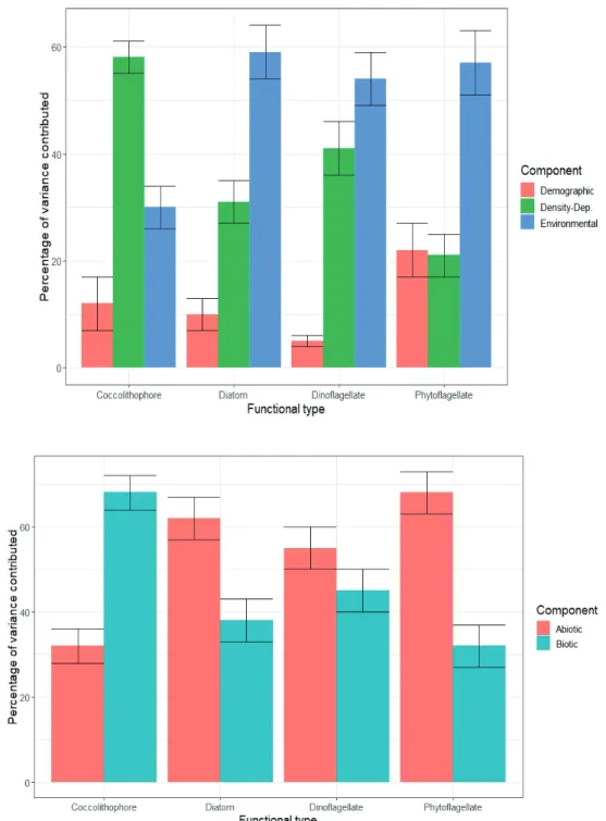
This facilitates the decomposition of the temporal variance in log-biomass growth of each group into additive contributions from different components. Accordingly, we use the reduced model to partition the temporal variance in the log-biomass dynamics of individual types into contributions from biotic factors, abiotic forcing and demographic stochasticity. We then introduce resource limitation and evaluate its contribution to temporal variation in the log-biomasses of individual groups by the subsequent reduction of the diagonal entries of the residual environmental covariance matrix C (the group- specific residual environmental variances).

Based on the reduced model where r_i,t = r_i, we decompose the total variance T_i in the log-biomass growth of the ith group over the study period as Ti = Gi + Ei + Di, where Gi, Ei

and D_i, and denote respectively the contributions of negative density feedback, environmental variability (including inter- specific interactions), and demographic stochasticity. Letting y_i represent the average log-biomass of the ith type over the study period, an estimate of demographic stochasticity in the log-biomass dynamics of the ith type at average log-biomass is

(6) If we denote by ni the temporal variance in the log-biomass of the ith type over the study period, and by x_q = (X_q,1, ..., X_q,T), then

(7)

(8) Since the forcing variables x_q = (q = 1, ..., Q) are mean-centered and standardized to unit variance, the formula for Ei

simplifies as

(9)

From the above variance partitioning, it follows that the proportion of temporal variation in the log-biomass growth of the ith group attributable to biotic factors (density-dependent regulation and pairwise interactions) is

(10)

The proportion of temporal variance in the log-biomass growth of the ith group due to environmental variability (including inter-specific interactions) is E_i/T_i. Similarly, the proportion of temporal variance in the log-biomass growth of the ith group due to density-dependent regulation is G_i/T_i and, at the average log-biomass of the ith group, the proportion of temporal variance in the log-biomass growth of the ith type due to demographic stochasticity is D_i/T_i. Alternatively, we can also separate the temporal variance in the log-biomass of the ith group excluding demographic stochasticity, (Ti – Di) in its abiotic and biotic components given by

respectively. We can also decompose the biotic component of temporal variation in the log-biomass of the ith group into contributions G_i from density-dependence and

from inter-specific interaction among types.

3. Application of the Bayesian model to the L4 phytoplankton community

3.1. Background

Phytoplankton is a generic name for a highly diverse group of photosynthetic organisms found in the euphotic zone of aquatic environments. As the base of the marine food web, phytoplankton sustain most of the aquatic life from zoo- plankton through fish to marine mammals (e.g., Doney 2006).

They also play a critical role in global biogeochemical cycles, particularly in the global carbon cycle through the “biological pump”, which accounts for roughly half of the total carbon fixation on Earth (Field et al. 1998). Therefore, identifying the factors and mechanisms underlying phytoplankton biomass dynamics and community structure and evaluating their relative importance is essential if we are to understand the

˘

8

from it. MCMC allow one to simulate the parameter(s) of interest from the correct posterior 203

distribution without the need to know its exact mathematical form. In practice, MCMC 204

simulation is conveniently implemented using freely available software packages such as 205

WinBUGS/OpenBUGS (Lunn et al. 2000, Thomas et al. 2006), JAGS (Plummer 2003), or Stan 206

(Stan �evelopment Team 2018). These software packages require the analyst to specify the 207

model in R-like code that the program uses to produce posterior MCMC samples according to 208

the prescribed prior distribution and likelihood or sampling distribution of the data at hand.

209

2.3. VARIANCE PARTITIONING 210

Based on the reduced model (2), the growth rate ∆𝑦�,� of the ith group can be expressed 211

as a linear function of the lagged log-biomasses 𝑦�,�� of all populations and coincident values 212

𝒙�= (𝑋�,�, . . ,𝑋�,�) of the environmental conditions under consideration at time 𝑡, with Gaussian 213

additive noise. This facilitates the decomposition of the temporal variance in log-biomass growth 214

of each group into additive contributions from different components. Accordingly, we use the 215

reduced model to partition the temporal variance in the log-biomass dynamics of individual types 216

into contributions from biotic factors, abiotic forcing and demographic stochasticity. We then 217

introduce resource limitation and evaluate its contribution to temporal variation in the log- 218

biomasses of individual groups by the subsequent reduction of the diagonal entries of the 219

residual environmental covariance matrix 𝑪 (the group-specific residual environmental 220

variances).

221

Based on the reduced model where 𝑟�,�=𝑟�, we decompose the total variance 𝑇�in the 222

log-biomass growth of the ith group over the study period as 𝑇_�=𝐺�+𝐸�+𝐷�, where 𝐺�, 𝐸� 223

and 𝐷�denote respectively the contributions of negative density feedback, environmental 224

variability (including inter-specific interactions), and demographic stochasticity. Letting 𝑦��

225

represent the average log-biomass of the ith type over the study period, an estimate of 226

demographic stochasticity in the log-biomass dynamics of the ith type at average log-biomass is 227

𝐷�=𝛿�/exp (𝑦��) (6)

228

If we denote by 𝑣� the temporal variance in the log-biomass of the ith type over the study period, 229

and by 𝒙�= (𝑋�,�, . . ,𝑋�,�), then 230

9 𝐺�=�^�_�^�

��^�𝑣� (7) 231

𝐸_�=∑ 𝛽��

� var�𝒙��+ �^�_�^�

��^�∑ 𝛼��

�� 𝑣_�+𝐶_�� (8)

232

Since the forcing variables 𝒙_� (𝑞= 1, … ,𝑄) are mean-centered and standardized to unit 233

variance, the formula for 𝐸_� simplifies as 234

𝐸�=∑ 𝛽� _��^� + �^�_�^�

��^�∑ 𝛼�� _��^�𝑣�+𝐶�� (9)

235

From the above variance partitioning, it follows that the proportion of temporal variation in the 236

log-biomass growth of the ith group attributable to biotic factors (density-dependent regulation 237

and pairwise interactions) is 238

𝐵_�= [𝐺�+ �^�_�^�

��^�∑ 𝛼�� _��^�𝑣�]/𝑇� (10)

239

The proportion of temporal variance in the log-biomass growth of the ith group due to 240

environmental variability (including inter-specific interactions) is 𝐸_�/𝑇�. Similarly, the 241

proportion of temporal variance in the log-biomass growth of the ith group due to density- 242

dependent regulation is 𝐺_�/𝑇� and, at the average log-biomass of the ith group, the proportion of 243

temporal variance in the log-biomass growth of the ith type due to demographic stochasticity is 244

𝐷�/𝑇�. Alternatively, we can also separate the temporal variance in the log-biomass of the ith 245

group excluding demographic stochasticity, (𝑇_�− 𝐷_�) in its abiotic and biotic components given 246

by ∑ 𝛽� _��^� +𝐶�� and 𝐺_�+ �^�_�^�

��^�∑ 𝛼�� _��^�𝑣�, respectively. We can also decompose the biotic 247

component of temporal variation in the log-biomass of the ith group into contributions 𝐺_� from 248

density-dependence and �_�^�^�

��^�∑ 𝛼�� _��^�𝑣� from inter-specific interaction among types.

249

3. Application of the Bayesian model to the L4 phytoplankton community 250

3.1. BACKGROUN�

251

Phytoplankton is a generic name for a highly diverse group of photosynthetic organisms 252

found in the euphotic zone of aquatic environments. As the base of the marine food web, 253

9 𝐺�=�_�^�^�

��^�𝑣� (7) 231

𝐸�=∑ 𝛽� _��^� var�𝒙��+ �_�^�^�

��^�∑ 𝛼�� _��^�𝑣�+𝐶�� (8) 232

𝐸�=∑ 𝛽��

� + �^�_�^�

��^�∑ 𝛼��

�� 𝑣�+𝐶�� (9)

235

𝐵_�= [𝐺_�+ �_�^�^�

��^�∑ 𝛼��

�� 𝑣_�]/𝑇_� (10)

239

dependent regulation is 𝐺_�/𝑇_� and, at the average log-biomass of the ith group, the proportion of 243

group excluding demographic stochasticity, (𝑇_�− 𝐷�) in its abiotic and biotic components given 246

by ∑ 𝛽��

� +𝐶_�� and 𝐺_�+ �^�_�^�

��^�∑ 𝛼��

�� 𝑣_�, respectively. We can also decompose the biotic 247

density-dependence and �^�_�^�

��^�∑ 𝛼��

�� 𝑣_� from inter-specific interaction among types.

249

3.1. BACKGROUN�

251

9 𝐺_�=�^�_�^�

��^�𝑣_� (7) 231

𝐸�=∑ 𝛽� _��^� var�𝒙��+ �^�_�^�

��^�∑ 𝛼�� _��^�𝑣�+𝐶�� (8) 232

𝐸�=∑ 𝛽��

� + �^�_�^�

��^�∑ 𝛼��

�� 𝑣�+𝐶�� (9)

235

𝐵_�= [𝐺_�+ �^�_�^�

��^�∑ 𝛼��

�� 𝑣_�]/𝑇_� (10)

239

environmental variability (including inter-specific interactions) is 𝐸_�/𝑇_�. Similarly, the 241

dependent regulation is 𝐺�/𝑇� and, at the average log-biomass of the ith group, the proportion of 243

by ∑ 𝛽��

� +𝐶_�� and 𝐺_�+ �^�_�^�

��^�∑ 𝛼��

density-dependence and �_�^�^�

249

3.1. BACKGROUN�

251

9 𝐺_�=�_�^�^�

��^�𝑣_� (7) 231

𝐸�=∑ 𝛽� _��^� var�𝒙��+ �_�^�^�

��^�∑ 𝛼�� _��^�𝑣�+𝐶�� (8) 232

𝐸�=∑ 𝛽��

� + �^�_�^�

��^�∑ 𝛼��

�� 𝑣�+𝐶�� (9)

235

𝐵_�= [𝐺_�+ �_�^�^�

��^�∑ 𝛼��

�� 𝑣_�]/𝑇_� (10)

239

dependent regulation is 𝐺_�/𝑇_� and, at the average log-biomass of the ith group, the proportion of 243

by ∑ 𝛽��

� +𝐶_�� and 𝐺_�+ �^�_�^�

��^�∑ 𝛼��

249

3.1. BACKGROUN�

251

9 𝐺�=�^�_�^�

��^�𝑣� (7) 231

𝐸_�=∑ 𝛽��

� var�𝒙��+ �^�_�^�

��^�∑ 𝛼��

�� 𝑣_�+𝐶_�� (8)

232

𝐸�=∑ 𝛽� _��^� + �_�^�^�

��^�∑ 𝛼�� _��^�𝑣�+𝐶�� (9)

235

𝐵_�= [𝐺�+ �^�_�^�

��^�∑ 𝛼�� _��^�𝑣�]/𝑇� (10)

239

dependent regulation is 𝐺_�/𝑇� and, at the average log-biomass of the ith group, the proportion of 243

by ∑ 𝛽� _��^� +𝐶�� and 𝐺_�+ �_�^�^�

��^�∑ 𝛼�� _��^�𝑣�, respectively. We can also decompose the biotic 247

��^�∑ 𝛼��

�� 𝑣� from inter-specific interaction among types.

249

3.1. BACKGROUN�

251

(5)

242 Mutshinda et al.

functioning of marine ecosystems and predict the structure of planktonic communities in a changing ocean (Irwin and Finkel 2018). Here we analyze the joint biomass dynamics of four major phytoplankton functional types namely, diatoms, dinoflagellates, coccolithophores and phytoflagellates using long-term monitoring data from a well-studied coastal station in the Western English Channel.

3.2. Description of data

We consider weekly observations of taxonomically re- solved phytoplankton biomass (mg C m^–3), along with co- extensive measurements of five environmental covariates recorded at 10 m depth in the upper mixed layer at Station L4 (50° 15.00′N, 4° 13.02′W) as part of the long-term Western Channel Observatory oceanographic time series (Widdicombe et al. 2010a,b). The data cover the period spanning 14 April 2003 through 31 �ecember 2009, a period over which all the re�uired data are available. Two of the five environmental variables under consideration namely, temperature (Temp,

°C) and salinity (Sal, PSU) describe water conditions. The temperature values range from 7.5ôC to 18.9ôC with a mean value of 13ôC, whereas all salinity values fall in a narrow range from 34.20 to 35.54 PSU with a mean value of 35.10 PSU (Fig. 1). The other three variables, photosynthetic active radiation (PAR; ), nitrogen concentration (Nit, ) and silicate concentration () characterize resource availability. Time- series plots of the five environmental variables at Station L4 over the study period reveal strong seasonal fluctuations (Fig.

1). Irradiance and temperature are highly correlated, but the two variables enter the model differently, which helps miti- gate potential identifiability issues.

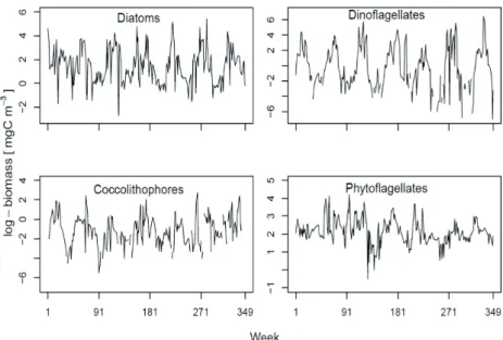
Phytoplankton biomass concentrations were calculated using taxa-specific biovolumes that were converted to carbon according to the equations of Menden-�euer and Lessard (2000) (Widdicombe et al. 2010b). For the purpose of the present study, we aggregate the phytoplankton into four functional types namely, diatoms, dinoflagellates, coccolithophorids and phytoflagellates and show the temporal variability of the natural log of each type’s biomass in Figure 2. Each group exhibits large variability both seasonally and inter-annually, with diatoms typically peaking in spring or early summer, while dinoflagellates are more common in summer. The coccolithophore biomass is highly variable and attributed to the dominance of the bloom-forming Emiliania huxleyi. The phytoflagellates dominated (more than 50% of the biomass) by unidentified flagellates less than 5µm in diameter show the least temporal variability relative to other functional types (Fig. 2).

3.3. Prior specification and model fitting

Before completing the model specification with explicit statements of priors on all unknown quantities, it is worth mentioning the postulated form of resource co-limitation to the growth rates of individual functional types in the full model. Following Mutshinda et al. (2017), we assume that the realized density-independent and resource-limited growth rate of the ith functional type from week w –1 to is given by r_i,w = m_if_i(w), where m_i > 0 is the maximum net growth rate of the ith functional type from one week to the next at average environmental conditions and optimal resource combination, and

(11)

26 715

716

Figure 1

717 718 719 720 721 722 723

724 725

Figure 1. Timeplots of the abiotic variables at Station L4 between April 2003 and �ecember 726

2009.

727

728 729 730 731 732

Figure 1. Timeplots of the abiotic variables at Station L4 between April 2003 and �ecember 2009.

11

Phytoplankton biomass concentrations were calculated using taxa-specific biovolumes that were 284

converted to carbon according to the equations of Menden-�euer and Lessard (2000) 285

(Widdicombe et al. 2010 b). For the purpose of the present study, we aggregate the 286

phytoplankton into four functional types namely, diatoms, dinoflagellates, coccolithophorids and 287

phytoflagellates and show the temporal variability of the natural log of each type’s biomass in 288

Figure 2. Each group exhibits large variability both seasonally and inter-annually, with diatoms 289

typically peaking in spring or early summer, while dinoflagellates are more common in summer.

290

The coccolithophore biomass is highly variable and attributed to the dominance of the bloom- 291

forming Emiliania huxleyi. The phytoflagellates dominated (more than 50% of the biomass) by 292

unidentified flagellates less than 5µm in diameter show the least temporal variability relative to 293

other functional types (Figure 2).

294

Insert Figure 2 Here 295

3.3. PRIOR SPECIFICATION AN� MO�EL FITTING 296

Before completing the model specification with explicit statements of priors on all 297

unknown quantities, it is worth mentioning the postulated form of resource co-limitation to the 298

growth rates of individual functional types in the full model. Following Mutshinda et al. (2017), 299

we assume that the realized density-independent and resource-limited growth rate of the ith 300

functional type from week 𝑤 −1 to 𝑤 is given by 𝑟�,�=𝜇� 𝑓�(𝑤), where 𝜇�> 0 is the maximum 301

net growth rate of the ith functional type from one week to the next at average environmental 302

conditions and optimal resource combination, and 303

𝑓�(𝑤) =𝑚𝑖𝑛 � 𝑃𝐴𝑅�

𝑃𝐴𝑅�+𝐾𝐸�, 𝑁𝑖𝑡�

𝑁𝑖𝑡�+𝐾𝑁�, 𝑆𝑖𝑙�

𝑆𝑖𝑙�+𝐾𝑆��

(11) where 𝐾𝐸�> 0, 𝐾𝑁�> 0 and 𝐾𝑆� > 0 denote respectively the irradiance, nitrogen and silicate 304

half-saturation constants representing the level of each resource at which 𝑟�,�=𝜇�/2, provided 305

that none of the other resources is limiting.

306

It is good practice to incorporate available information into the analysis by specifying 307

informative prior distributions for some of the model parameters, which can greatly improve 308

the estimation precision (�elean et al. 2013). Based on our previous experience with the L4 data 309