T Comparing the IMF and the ESM through Bond Market Premia in the Eurozone

(1)

T

Gábor Dávid Kiss – Máté Csiki – János Zoltán Varga

Comparing the IMF and the ESM through Bond Market Premia in the Eurozone

Summary: In many European Union (EU) member countries, the financial turmoil that started in 2008 resulted in a banking and/

or sovereign debt crisis. The EU did not have dedicated tools to handle the situation and it became clear that neither the IMF loans, nor the ad hoc intergovernmental loans provided satisfactory solutions. This motivated the establishment of the Euro- pean Stability Mechanism (ESM). In this study, we compared the lending activity of the IMF and the ESM, their institutional background, and using panel regression methods we investigated the effect of EFSM-ESM loans on monthly sovereign bond yield premia. Results: The ESM programmes worked against bond market divergence, yield premia decreased, and they moved more closely together – which is a precondition of an efficient eurozone-wide monetary policy. Since EFSM-ESM bonds are guaranteed by euro area member states, it fulfils the solidarity principle of the optimum currency area, and with the help of EFSM-ESM programmes, sovereign defaults have been successfully avoided.

K^eywordS: monetary policy, International Financial Markets, International Lending and Debt Problem, Panel Data Models JeL ^codeS: C23, E52, F34, G15

The eurozone, created by the core states of the european union, did not have an institutional and financial background to deal with banking and sovereign debt crises at the time of its establishment. Because of this, member states tried to handle the effects of the global financial crisis that started in 2008 with funds from the international Monetary Fund (iMF) and ad-hoc intergovernmental loans at first.

Later it became clear that this was insufficient, both politically and financially, and that a permanent, dedicated fund was required, so the european stability Mechanism (esM)

was created. in this study we compare the iMF, an institution with a history of nearly 75 years, and the esM, established with an intergovernmental treaty after 2012, and we explore the effects of the esM on bond markets.

Programmes to transform the esM into a

‘european Monetary Fund’ as we see it in Jean- Claude Juncker’s ‘sixth scenario’ and in com- munication from the european Commission in 2017¹ and the Managing director of the esM in 2018², also prompt a comparison of the two multilateral funds used for crisis management (Losoncz, 2017).

in case of the iMF, the obligation of con- vertibility according to section (4) of Arti- E-mail address: kiss.gabor.david@eco.u-szeged.hu

(2)

cle Viii of the Articles of Agreement needs to be highlighted, as its aim these days is to ensure the free movement of capital and thus financial account liberalisation. Meanwhile the esM, with a reverse approach, provides an institutionalised solution for easing the tensions caused by the liberalisation of capital movements. it is important to state, however, that these organisations can only manage certain crises, acting like a firewall to stop them from spreading (Báger, 2017), considering that in a country with a population of several million, it takes a lot of economic and political inter- actions to create and to come out of a crisis.

The present paper focuses only on the eurozone countries: we examined the changes in the long term bond market yields with monthly time-series between 2006 and 2018, looking for factors that work against the divergence caused by the crisis, using a dynamic panel regression model.

in our study, an overview of how the esM was created is followed by a comparison of the framework of the lending activities of the iMF and the esM, then we present the data and methodology used for the empirical analysis, and finally we assess the results and draw the conclusions.

ThEoRETICaL baCkGRoUnD

if a state is not able or not willing to meet its payment obligations, it typically can’t sell the sovereign bonds meant to finance government deficits and maturing sovereign debt at a reasonable yield, and there are problems with interest payment as well (Losoncz, 2014). in this case, the options include rescheduling with the same present value, restructuring while decreasing the present value, and partial remittance. The country in trouble can negotiate with its sovereign creditors within the Paris Club and with its private creditors

in the London Club (if it is not too atomised).

Another option is to take intergovernmental loans, provided there is a willing partner. After the Bretton Woods conference (1944), the iMF became the institutionalised framework for sovereign multilateral lending. The iMF can diversify the sources of financing and lending, and it has the competencies to set the conditions of the latter. This means that when a country switches to iMF financing from market financing, it is at the expense of the collective sovereign debt of the iMF member states.

A sovereign default may easily lead to a banking crisis and vice versa: as the default risk of sovereign bonds increases, it jeopardises the solvency and liquidity of the banking system, while a too costly bank consolidation may lead to a situation where sovereign bonds are hard to sell on a market that has liquidity problems in the first place. A capital increase meant to absorb the credit losses of the banking system can easily get stalled, or, with surging sovereign debt, it may also drag down the country concerned (Botos, 2006; Botos, 2014; Laeven, 2011; Reinhart et al., 2011).

The european stability Mechanism (esM) was established in 2012³ with an international treaty outside of eu legislation (as con- firmed later by the european Court of Justice in the Pringle case) to protect the stability of the eurozone, as an instrument of economic policy (Kálmán, 2016; Benczes, 2014; Várnay, 2016). The eurozone must ensure free capital flow, which stems from the theory of Op- timum Currency Area (Mundell, 1961), and at the same time, resulting from the impossible trinity, it must also ensure irreversibly fixed exchange rates and the maintenance of a common monetary policy, while there are provisions against exit, no bailout and sovereign default (Losoncz, 2017; Marján, Buda, 2014;

Benczes, 2011). The free flow of capital is es- sential, so we will examine this from two as-

(3)

pects: how it brought the idea of a banking union to centre stage and how this effects the convergence of bond market yields.

due to free capital flows and the free pro- vision of services, financial crises spread more easily through parent banks (Árvai et al., 2009) and the balance sheet total of certain bank groups are now comparable to the gross national product of member states. Because of this, the aim of macroprudential policy⁴ is to mitigate system-level crises, to prevent excessive credit growth, to manage liquidity risks and to avoid excessive risk-taking. This is also the aim of the Banking union, which focuses mostly on the eurozone but is also open to other member states, through the direct supervision of banks that are significant on a system-level (single supervisory Mechanism), and through the common resolution fund and deposit insurance fund (Mérő, 2017). some of the resources provided by the esM, described in the following sections, were also spent on bank consolidation by the recipient countries, which, again, underlines the significance of the institutional deepening mentioned before.

in our work we focus on the effects of the introduction of the esM on bond markets.

The Maastricht criteria⁵, on which the eurozone is based, included the requirement of the convergence of long-term bond yields. Bearce (2002), however, raised the possibility of a reverse process (the divergence of yields). Con- sidering that members of the eurozone issue sovereign bonds with different credit ratings (anywhere between B- and AAA ratings), a global decline in risk-appetite may lead to a safety trap, increasing demand for low-risk assets, resulting in their near-zero returns (Hor- váth, szini, 2015). This, in itself, may increase the yield spread over member states with AAA rating.

Bond yields must be affected by the transmission mechanism of monetary policy as well, both in case of repo and final purchase

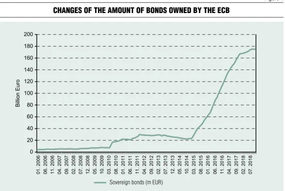
transactions. Along with near-zero key interest rates, the european Central Bank (eCB) introduced longer repo operations at first, then, from 2010, together with member state central banks⁶, it had a series of bond purchase programmes that covered asset-backed securities (ABs)⁷, residential and commercial mort- gage-backed securities (MBs) and sovereign bonds purchased on secondary markets – especially after 2015.^{8, 9} Figure 1 shows the changes of the amount of bonds owned by the eCB.

in addition, the eCB purchases sovereign bonds in the Outright Monetary transactions (OMt) programme if the eurozone member state concerned receives esM (or previously eFsF) financing according to a Memorandum of understanding that the state concluded earlier with the Commission and if it complies with the economic policy provisions laid down in it (Várnay, 2016).

This means that if we want to examine how the esM affects bond yields, we need to take a look at the eCB’s bond purchase programme as well, which is best illustrated by the increasing amount of bonds in the balance sheet of the central bank.

Comparing the IMF and the ESM

it makes the institutional background even more complex that the european Commission has always involved the iMF as a partner in the crisis management process (Marján, Buda, 2014; Losoncz, 2014). This involvement is justified by the high quota of the eurozone member states, their considerable voting power and credit facilities. in the iMF, according to the latest, fifteenth amendment accepted in 2008, it is a 19 percent quota share¹⁰ (us 14.7 percent), which is sdR 103.8 bn. in addition, euro area countries contribute to the NAB (New Arrangements to Borrow) and GAB (Ge- neral Arrangements to Borrow) funds, which

(4)

constitute the source of financing for the iMF, with 36 percent and 26 percent respectively.¹¹ Which means it would not be rational not to rely on these available resources.

On the other hand, except for the recon- struction after the second world war and some short detours (and the support provided to countries during the political transition of the 1990s), the iMF did not focus on european and euro area countries. Considering this, it is understandable that the ecofin and the european Commission became committed to the establishment of an own crisis management fund (more than one, with the bank resolution fund). Another important difference is that the esM admittedly has no independent decision-making powers, it is only responsible for the availability of funds [an 85 percent majority of members is required for access (Móra, 2013)].

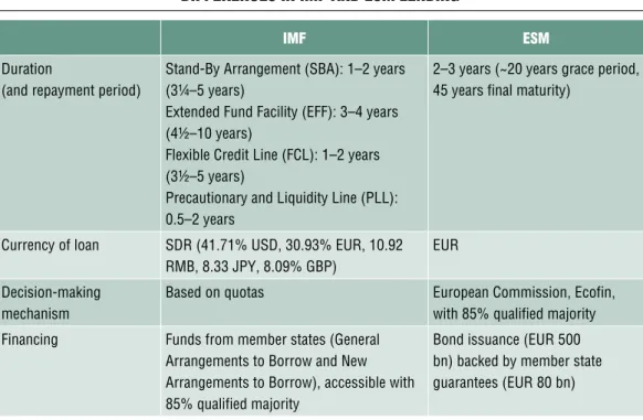
The iMF lends the resources provided by the member states for a maximum duration of ten years, while the esM can set a 50 year repayment period for its loans, for which it rais- es capital from the bonds it issues with member state guarantees. This is also useful from the aspect of how sovereign debts affected by the consolidation are spread over time. Table 1 shows the main differences between the lending facilities.

esM bonds are officially recognised as bonds issued by a sovereign, supranational Agency (ssA), which receive a 0 percent risk weight according to the Basel ii document¹². in addition, the european Banking Authority recognises it as an ‘extremely high quality liq- uid asset’, and it is accepted by the eCB and the Bank of england as collateral. esM sells bonds globally through 41 institutional investors, while short-term notes provided for the

Figure 1 Changes of the amount of bonds owned by the eCb

Source: edited by the authors based on the ECb statistical database Sovereign bonds (m EUR)

(5)

recapitalisation of the banking sector may only be used in the repo markets as collateral.¹³ The interest rates of the bonds issued are built in the interest rates of the loans provided to the recipient countries, together with the commission that ensures the operation of the esM and the stand-by fee.

The lending facility of the eMs can be seen as some ‘bad eurozone bond’, and its ac- ceptance is sweetened by the related sovereign guarantees, the solvency capital requirement benefits and the fact that they are accepted as collateral (sági, 2018). From an institutional aspect, it seemed an acceptable hybrid solution in addition to the politically less popular other options, namely ad-hoc bilateral loans, the ‘euro bond’ covering the whole euro area, and the bonds issued by the european Com- mission (european Financial stabilisation

Mechanism). The establishment of the esM, however, clearly indicated that in addition to the emergency reforms of the stability and Growth Pact, member states were ready for showing solidarity that complies with the pro- hibition of sovereign default and for a deepening integration (Benczes, Rezessy, 2013; Kuta- si, 2012). it is a question, however, also raised by Benczes and Rezessy (2013), and Vigvári (2015), what will happen if a larger member state gets into trouble.

Member states receiving ESM funding

The esM provides funding to member states through several channels: conventional loans (to ireland, Portugal, Greece and Cyprus), loans for the recapitalisation of the bank-

Table 1 differenCes in imf and esm lending

imf esm

Duration

(and repayment period)

Stand-By Arrangement (SBA): 1–2 years (3¼–5 years)

Extended Fund Facility (EFF): 3–4 years (4½–10 years)

Flexible Credit Line (FCL): 1–2 years (3½–5 years)

Precautionary and Liquidity Line (PLL):

0.5–2 years

2–3 years (~20 years grace period, 45 years final maturity)

Currency of loan SDR (41.71% USD, 30.93% EUR, 10.92 RMB, 8.33 JPY, 8.09% GBP)

EUR

Decision-making mechanism

Based on quotas European Commission, Ecofin,

with 85% qualified majority Financing Funds from member states (General

Arrangements to Borrow and New Arrangements to Borrow), accessible with 85% qualified majority

Bond issuance (EUR 500 bn) backed by member state guarantees (EUR 80 bn) Note: without loans to poor countries

Source: IMF, ESM websites

(6)

ing system (spain); the programme in which sovereign bonds are purchased on the primary and secondary markets and the precautionary liquidity line have not yet been used. in this subsection we describe the use and maturity profile of loans provided through the eFsF/

esM, relying on data from the website of the organisation.

Greece returned to full market financing in 2018 after the first loan agreement was made in 2010 to manage the crisis. in this agreement Greece first received bilateral loans of euR 52.9 bn and a loan of euR 20.1 bn from the iMF, which was followed by a euR 141.8 bn eFsF (and a euR 12 bn iMF) package between 2012 and 2015, then an additional amount of euR 61.9 bn was allocated within the esM. in the case of the eFsF, it must be emphasised how the private sector (especially banks) were involved in crisis management: in May 2012, 97 percent (euR 197 bn) of pri- vately owned bonds were subject to a 53.5 percent haircut, in which Greek sovereign bonds were swapped with eFsF bonds, the maturity of which was later extended. After that, 55 percent of Greece’s sovereign debt was held by the esM, with an average maturity period of 32.25 years and a 2034–2060 repayment period. in November 2018, a decision was made to extend the weighted average maturity of all eFsF loan tranches by ten years, which, together with the low variable borrowing rates (average: 1.62 percent), may result in significant debt reduction by 2060.¹⁴ 58 percent of esF funds were spent on debt servicing, 18 percent on building a cash buffer, 11.3 percent on arrears clearance and 8.7 percent on bank recapitalisation.

Cyprus first received a loan from the iMF (euR 1 bn) in 2012, then from the esM (euR 6.3 bn), with an average maturity period of 14.9 years. The repayment period is from 2026 to 2031, the average variable borrowing rate is 0.91 percent. euR 1.5 bn of the

loans was used for the recapitalisation of the banking system.

Portugal needed iMF-eFsF-esM support between 2011 and 2014, receiving euR 26 bn from each, and euR 12 bn of this was used for the recapitalisation of three large banks. Bor- rowing rates vary, the average rate is 1.76 percent, the average maturity period is 20.8 years, the repayment period is between 2025–2040.

From 2010 to 2012, ireland needed loans from the iMF (euR 22.5 bn), the european Commission (euR 22.5 bn), the eFsF (euR 17.7 bn), the united Kingdom (euR 3.8 bn), sweden (euR 0.6 bn) and denmark (euR 0.4 bn). The average maturity period of the eFsF loans is 20.8 years, the repayment period is between 2029 and 2042, and most recently the variable borrowing rates were at 1.79 percent. The funds were mostly used for financing the budget deficit, and a smaller part was used for the recapitalisation of the banking system.

spain only used esM funds for the recapitalisation of the banking system. The total amount between 2012 and 2013 was euR 41.3 bn, with maturity between 2025 and 2027 (the average variable interest rate is 1.11 percent), capital repayment starts in 2022, but euR 17.612 bn has already been repaid vol- untarily. The iMF was not involved, as at the time it did not have facilities suitable for the recapitalisation of the banking system. esM funds were managed by the restructuring fund of the spanish government, Fondo de Ree- structuración Ordenada Bancaria, and it involved 8 banks. An asset management fund was also established.

Overall, the esM provided loans with variable interest rates (with the exception of the facility provided to Greece, amended in 2018), not exposing itself to market interest risks. On the other hand, it launched programmes that span over decades, sometimes 50 years, and the economic policy of the recipient countries are

(7)

now under strict supervision until 75 percent of the loans are repaid (Ódor, P. Kiss, 2011;

török, 2018). every member state involved in these assistance programmes managed to re- turn to direct capital market financing, which suggests the programme is accepted.

METhoDoLoGy, MoDEL anD DaTa

in our study we used GARCH models to model the autoregression and heteroskedasticity of the time series, used the dynamic conditional correlation (dCC) model to analyse the correlation of bond market yields, and we used dynamic panel regression on monthly bond market data to analyse how the allocation of the eFsF-esM funds influenced the change in yield premia over the German benchmark.

When iMF or esM financing is used, the state concerned replaces bond market financing, partially or wholly, with international financing, then it later returns to market sources. to serve domestic private and institutional investors (the banking system, insurance com- panies, investment funds, etc.) bond markets need to be sustained in the course of these programmes, and the changes in the yields there clearly indicate the market’s assessment of the viability of the consolidation programme.

Model

Based on Bearce (2002), we talk about bond market divergence if the yield spread starts to increase, meaning market operators stop considering the eurozone as a homogeneous unit. Considering the strength of the German economy and the AAA rating of German sovereign bonds by s&P, it is useful to calculate yield premia over those. The change of the yield premia may considerably depend on its own past value (we can assume there is

autocorrelation) and on the change in the co- movement of the two yields. The conditional standard deviation of the bond yield may also be important, as it expresses the uncertainty of pricing. The sovereign debt financing by the eFsF-esM and the bond purchases of the eCB (which fine tune monetary policy transmission) should also be examined.

Our model takes all this into consideration and is as follows:

∆ln(r_d–r_DE)_t= α∆ln(r_d–r_DE)_t–1 + ω + β∆DCC_d–DE,t+ γ∆σ_d,t+ δdummy_ESM,t

+ μdummy_IMF,t+ θ∆lnECB_t+ ε_t (1) Where ∆ln(r_d–r_DE) is the logarithmic change of the yield premium over German sovereign bonds,¹⁵ ω is the constant, ∆DCC_d–DE,t is the change of the dynamic conditional correlation calculated with German sovereign bonds ∆σ_d,t is the change of conditional standard deviation, the fact that esM or earlier eFsF sources were used¹⁶ is expressed with the dummy variable δdummy_ESM,t, the existence of iMF funds is expressed by the μdummy_IMF,tdummy variable, ∆lnECB_tis the logarithmic change of the amount of sovereign bonds in the balance sheet of the eCB, and ε_tis the error term.

Based on the assumptions, the loosening of the previous close co-movement of yields is expected to result in an increase in the yield premium, and similarly, in an increase in the standard deviation (riskiness) of bond yields.

The funds regularly transferred by the eFsF- esM and the eCB’s sovereign bond purchases were meant to counterbalance this process.

The methodology of dynamic panel regression

Cross-sectional analyses at a certain point in time often lead to distorted and inconsistent estimates. using panel data, we can examine

(8)

the dynamics of the effects as well, getting a more accurate picture of the effects of the processes that evolve in space and time.

unobserved time invariant and/or individual invariant factors may result in endogeneity, which can be filtered out with adding fixed effects to the model (Balázsi et al., 2014).

Our sample contains every country that has an effect on the research question, so it is not a random sample, which also calls for the application of the fixed-effect model (Judson, Owen 1999).

if the result variable (y_it) is autocorrelated, the result variable’s (y_it) lagged values (y_it–1) need to be added to the regression equation as an explanatory variable (Balázsi et al., 2014).

ignoring the autocorrelation of the result variable would be a mistake similar to leaving another important explanatory variable out from the model. so it is the relatively large number of observed variables, the relatively short time series and the presence of the autocorrelated result variable that calls for the use of dynamic panel models. As opposed to stat- ic panel models, dynamic panel models use the lagged values of the result variable as an explanatory variable. using a lagged dependent variable as a regressor is contrary to strict exogeneity, as the lagged dependent variable is necessarily correlated with the error term, and as a result the techniques used in stat- ic models like fixed-effect estimating func- tions lead to inconsistent estimates. if some fixed-effect structure is inserted in a dynamic model, the resulting estimating function results in an inconsistent estimate in N (number of observations) for a fixed T (length of the time series) (Balázsi et al., 2014). to deal with this, in our study we used the following dynamic panel regression, based on Arel- lano and Bond (1991). The GMM procedure of Arellano and Bond (1991) uses all available lags as the instruments of the differenced lagged dependent variable.

The relatively large number of observed variables, the relatively short time series and the presence of the autocorrelated result variable call for the use of dynamic panel models. The method is based on an AR(1) process, where, to deal with the problem of endogeneity, the result variable y_it is explained by its own lagged values, using the variable specific μ_i and the zero mean value v_it uncorrelated error terms as customary with fixed effect panel regressions (Blundell, Bond, 1998; Arellano, Bond, 1991):

y_it= αy_it–1+ μ_i+ v_it, i=1,…, n, t = 1,…, T_i. (2) Which is supplemented by the introduction of the explanatory variables in the model:

y_it= αy_it–1+ βx_it+ μ_i+v_it, i = 1,…, n, t = 1,…, T_i. (3) with the following restrictions:

y_it= βx_it+ f_i+ ξ_it, where ξ_it= αξ_it–1+ v_i

and μ_i= (1–α) f_i, |α|<1. (4) Overidentification occurs when there are more variables in the model then required for the estimation. The potential overidentification of the model was tested with the sargan test, the null hypothesis of which states that model parameters are identified via a priori restrictions on the coefficients (if p>0.05, the output is acceptable).

GARCH models

Problems arising from autoregression and heteroskedasticity are mostly handled with the generalised ARCH models, i.e. the GARCH (Generalised Autoregressive Conditional Heteroskedasticity) models. in the GARCH(p, q) model p and ε² represent the lookback period of the error term, q and σ²represent

(9)

the lookback period of standard deviation, α_i represents the effects of current news on conditional variance, and β_i represents volatility persistence, i.e. the shock of current news on past information (Kiss, 2017):

σ_t²= ω + ∑ ^p_i=1 α_i ε²_t–i + ∑ ^q_i=1 β_i σ ²_t-i. (5) The basic GARCH(1,1) model assumes that present volatility depends on past volatility and yields, and that there is no difference between market reactions to positive and negative shocks. With asymmetric GARCH models – for example: GJR-GARCH – the leverage effect can be introduced to the model, which states that negative yields (losses) are more frequently followed by volatile periods.

The significance of asymmetry is to grasp the stronger reactions to negative news. The GJR- GARCH model defines asymmetric reactions with an S dummy variable (Kiss 2017):

{

^S^S^–^t-i^–t-i ⁼= ^{1, ha ε}0, ha ε^t–i_t–i^<≥ ⁰0, (6) where the GJR-GARCH(p,o,q) model can be written as follows:

σ²_t = ω + ∑^p_i=1 α_i ε²_t–i + ∑^o_i=1 γ_i S ^–_t–1 ε ²_t–i +∑^q_i=1

β_i σ ²_t–i, (7)

where α₁ > 0 (i=1,…, p), γ_i+α_i> 0 (i=1,…,o), β_i ≥ 0 (i=1,…,q),α_i+ 0,5 γ_i+ β_k< 1 (i=1,…, p, j = 1,…, o, k = 1,…,q). Based on the minimum value of the Bayesian information Criterion (BiC), calculated with the maximum likelihood estimation, we optimised every possible combination of the values of the p, o and q parameters (p=1,2; o=0,1; q=1,2), and as a result, in 58 percent of the cases it was the GJR-GARCH(1,1,1) model, in the other 42 percent it was the GARCH(1,1) model that fit optimally. For the sake of comparability, we used the estimations

of the GJR-GARCH(1,1,1) model on the whole sample.

to demonstrate the convergence or divergence of bond yields, the change of correlation over time needs to be verified, for which the suitable tool is the dynamic conditional correlation model (dCC-model(1,1,1)), by which heteroskedasticity can be modelled.

Based on Engle (2002), the dynamic conditional correlation model (dCC model) models the conditional σ²_it variance of time series with a r_t‖ Φ_t–1~N(0,H_t ] yield and Φ_t–1 information available at any t–1 time:

[

^σ^σî,j,t²î,t^σ^σî,j,t²^j,t

]

^{= ∑}^pⁱ⁼¹^α^i,j

[

êê²î,t–pî,j,t–p êêî,j,t–p²î,t–p

]

⁺

+ ∑^q_i=1 β_i,j

[

^σ^σî,j,t–q²î,t–q^σ^σî,j,t–q²^j,t–q

]

⁽⁸⁾

where the i=1:N–1 index is the logarithmic change of the 10-year bonds of the euro area states, and the j=N index is the logarithmic change of German 10-year bonds.

Presentation of data

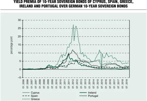
data from the eCB statistical database are monthly data between January 2006 and November 2018 regarding 10-year sovereign bonds. From this, we first we calculated the recipient countries’ yield premia over German 10-year bonds. Figure 2 shows the yield premia of the countries in the eFsM- esM programme. As a result of the 2008–

2009 global financial crisis, its repercussions and the sovereign debt crisis of the eurozone, the yield premia of the peripheral countries of the eurozone increased significantly.

There was a risk that strongly rising yields unjustified by fundamentals in the countries that were the most affected by the debt crisis would lead to a self-fulfilling sovereign crisis,

(10)

i.e. to a situation where rising yields on their own, in parallel with high outstanding debts, significantly impair the sustainability of sovereign debt (Krekó et al., 2012). in case of yield premia, the largest surge was in Greece, while it was spanish yields that stayed the closest to German yields. After 2012, the effects of the crisis management of the iMF and the institutionalised crisis management of the eurozone were visible, and so were the effects of the non-conventional monetary policy tools of the eCB, which helped decrease the yield premia of the countries on the periphery.

The eCB announced its securities Mar- kets Programme (sMP) in May 2010, following a significant increase in the premia of longer-term sovereign bonds in euro area periphery countries (Krekó et al., 2012). With-

in the sMP, the eCB purchased long-term sovereign bonds for euR 218 bn (Ghysels et al., 2014). The sMP was successful in the short term, as the yields of long term sovereign bonds decreased in the vulnerable econ- omies of the eurozone, but the long term effects of the programme cannot be separated from other market effects (Krekó et al., 2012;

Ghysels et al., 2014). in addition, the eCB launched its largest-scale asset purchase programme to date in early 2015: in the APP (ex- panded asset purchase programme), significant amounts of eurozone sovereign bonds were purchased.

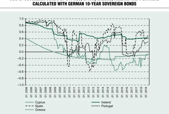
Figure 2 shows the yield premia of the 10- year sovereign bonds of the recipient countries, Cyprus, spain, Greece, ireland and Por- tugal, over German 10-year sovereign bonds, while Figure 3 shows the dynamic condition-

Figure 2 yield premia of 10-year sovereign bonds of Cyprus, spain, greeCe,

ireland and portugal over german 10-year sovereign bonds

Source: ECb, own calculation

percentage point

(11)

al correlation of the German sovereign bond, modelled with the dCC-procedure. An exam- ination of the co-movement of sovereign bond yields reveals that the 2008 financial crisis significantly disrupted the yield convergence that characterised the pre-crisis period. As the debt crisis deepened in europe, the sovereign bond yields of the periphery countries diverged from German sovereign bonds, with significant volatility (sági, 2012). in most countries examined (except for ireland) there were periods with negative co-movement occurred (in opposite directions). in Greece, this negative co-movement was of lasting nature, which was mostly caused by the steadily high yield premia. The yield of the sovereign bonds of Cyprus was less convergent before the crisis, and after the crisis there was a long term, slight, negative co- movement.

to deal with problems arising from autoregression and heteroskedasticity, we fit the GJR-GARCH model on the elements of the time series that contained the bond yields of the countries examined. The asymmetric GJR-GARCH(1,1,1) model was necessary for the bond yields, where the number of lags is 1 for innovation, asymmetry and volatility. it is clear from Figure 4 that the conditional standard deviation of bond yields significantly increased after the crisis, especially in the case of Greek and irish 10-year sovereign bonds. Af- ter 2015, as a result of the market uncertainty around the eurozone, the ongoing Greek debt crisis and the non-conventional tools (expand- ed asset purchase programme, APP) used to manage these situations, the conditional volatility of the bond yields increased in the countries examined.

Figure 3 dCC of sovereign bonds of Cyprus, spain, greeCe, ireland and portugal

CalCulated with german 10-year sovereign bonds

Source: ECb, own calculation (Matlab, MFE toolbox)

(12)

in the case of the sovereign bonds of Cy- prus, we can see that the conditional standard deviation returns to the expected value – we got the same results with the alternative GARCH(1,1) model¹⁷, which suggests that the result is characteristic of the time series.

This, however, had an impact on the results of the dCC as well.

RESULTS

We ran the model on the original monthly time series, and on the averaged quarterly time series calculated from that to compensate for the distortion caused by the discrete capital transfers provided by the esM (see Table 2).

The sample covered the whole eurozone, and we also examined the panel with the countries

participating in the eFsF-esM-programme.

From the coefficients in the dynamic panel regressions, the ones with positive value represent the variables encouraging divergence, and the ones with negative value represent the variables encouraging convergence.

Based on table 2 we can establish that the model applied is correct, as the increase in the correlation led to the decrease in the yield premia over German sovereign bonds – meaning there was convergence (d_DCC variable).

Meanwhile the increase in the conditional standard deviation calculated from the logarithmic change of the bond yield typically resulted in the decrease of the premium (d_standardde- viation variable).¹⁸ The existence of eFsF-esM transfers also had a decreasing effect on yield premia, which means it worked against divergence. According to the model, the funds re- Figure 4 Conditional standard deviation of bond yields –

gJr-garCh(1,1,1)

Source: ECb, own calculation (Matlab, MFE toolbox)

(13)

ceived through the eFsF-esM achieved their theoretic effect, they had a decreasing effect on the yield premia over German sovereign bonds in the recipient countries, contributing to the sustainability of the sovereign debt financing of the countries examined (dummy-ESM variable). The effect of iMF resources can only be detected in the monthly data; in this case, the presence of iMF resources decreased the yield premia over German sovereign bonds, i.e. they

led to the convergence of yield levels (dummy_

IMF variable). in a peculiar way, the dln_ECB variable, which represents the increase in the amount of sovereign bonds held by the eCB, contributed toward divergence in every case – this effect needs to be explored separately, which is beyond the scope of this study.

it needs to be emphasised that there is no significant difference between the results from monthly and quarterly data, and between the Table 2 Changes in the bond market premia of member states partiCipating

in the efsf and esm programmes

Quarterly data monthly data

total esm total esm

variable coefficient p-value coefficient p-value coefficient p-value coefficient p-value

dln_premium –0.0497 0.4965 –0.0750 0.3621 –0.0481 0.418 0.1829 0.0003***

Constant –0.0052 ^0.0000*** –0.0087 ^0.0000*** –0.0007 ^0.0000*** –0.0006 0.0000***

d_DCC –0.1443 ^0.0000*** –0.1567 ^0.0006*** 0.0213 ^0.6657 –0.0397 0.2025 d_standard-

deviation

–0.3579 ^0.0000*** –0.9515 ^0.0397** –0.4201 ^0.0001*** 0.4545 0.0019***

dummy_ESM –0.0979 0.0000*** –0.0953 0.0000*** –0.0247 0.0502* –0.0123 0.4342 dummy_IMF –0.0967 ^0.3452 –0.0887 ^0.4036 –0.0361 ^0.0000*** –0.0217 0.0271**

dln_ECb 0.1240 ^0.0215** 0.0987 ^0.2593 0.2530 ^0.0000*** 0.1478 0.0362**

Sargan test ^0.5276 ^0.3318 ^0.9995 0.8001

corr(d_DCC,res) 0.07 0.07 0.05 0.09

corr(d_standard- deviation, res)

0.07 0.00 0.09 0.06

Note: the structure of the applied model was as follows: ∆ln(r_d–r_DE )_t = α∆ln(r_d–r_DE)_t–1 + ω + β∆DCC_d-DE,t + γ∆σ_d,t + δdummy_ESM,t + μdummy_IMF,t + θ∆lnECB_t + ε_t. Where ∆ln(r_d–r_DE )_t is the logarithmic change of the yield premium over German sovereign bonds, ω is the constant, ∆DCC_d-DE,t is the change of the dynamic conditional correlation, γ∆σ_d,t is the change of conditional standard deviation, the fact that ESM or earlier EFSF sources were used is expressed with the dummy variable δdummy_ESM,t, the IMF funds are expressed with the dummy variable μdummy_IMF,t, ∆lnECB_t is the logarithmic change of the amount of sovereign bonds in the balance sheet of the ECb, and ε_t is the error term. If p<0.1 then *, p<0.05 then **, p<0.01 then ***.

The d_DCC and d_standarddeviation variables are uncorrelated with the error terms of the regression, so there is no endogeneity bias.

Source: edited by the authors, Gretl

(14)

samples covering the whole eurozone and the eFsF-esM programme countries, meaning they are sufficiently robust.

SUMMaRy

in our study, we compared the operation of the esM and the iMF, based on their crisis management in the eurozone. We explored institutional differences and the different financing channels, and we provided a brief description of the background of the financing facilities provided to the countries in the programme. Then we used bond market

data to analyse how the allocation of eFsF- esM funds influenced the change of the yield premia over the German benchmark.

We established that the esM programme acted against bond market divergence, the yield premium over German sovereign bonds decreased, and their co-movement increased, which is a precondition of a monetary policy that covers the whole euro area. With these measures the no-default rule, on which the eurozone is based and which is the financial man- ifestation of solidarity as presented in the optimum currency area theory, was sustainable, as the eFsF-esM bonds are guaranteed by the eurozone member states.

Notes

1 https://ec.europa.eu/commission/sites/beta-political/files/reflection-paper-emu_en.pdf

2 https://www.esm.europa.eu/speeches-and-presen- tations/european-monetary-fund-what-purpose- speech-klaus-regling

3 Which replaced the european Financial stabilisation Mechanism established in 2010 (Council Regulation (eu) No 407/2010) and the european Financial stability Facility.

4 http://www.mnb.hu/en/financial-stability/macroprudential-policy/a-brief-review-of-macro prudential-policy

5 treaty Article 109j (1).

https://europa.eu/european-union/sites/europaeu/

files/docs/body/treaty_on_european_union_

en.pdf

6 in proportion to the eCB shares they own.

7 http://www.ecb.europa.eu/ecb/legal/pdf/oj_

jol_2015_001_r_0002_en_txt.pdf

8 http://www.ecb.europa.eu/press/pr/date/2015/

html/pr150122_1.en.html

9 http://www.ecb.europa.eu/ecb/legal/pdf/en_dec_

ecb_2015_10_f_.sign.pdf

10 https://www.imf.org/external/np/fin/quotas/

2018/0818.htm

11 http://www.imf.org/external/np/exr/facts/gabnab.

htm

12 https://www.bis.org/publ/bcbs_nl17.htm

13 https://www.esm.europa.eu/investors/esm/funding- strategy

14 https://www.esm.europa.eu/press-releases/explainer- efsf-medium-term-debt-relief-measures-greece

(15)

15 The yield premium was logarithmised to improve the scalability of the output, and in 98.5 percent of cases, it had a positive value. For the other 1.5 percent of cases, mostly from 2006, we used zero values.

16 time series on the side of the esM contain too discrete capital movements, and they are difficult to fit in a time series with monthly or quarterly data.

17 The correlation of the conditional standard deviation obtained from the two models is 0.9991.

18 This result is somewhat counterintuitive, but it subsisted when the model was run with different sets of variables (e.g. without the iMF dummy), so probably it is because the surge in the conditional standard deviation coincided with the decrease in yields, which underlines the necessity to use the asymmetric GARCH model.

References Árvai, Zs., driessen, K., Ötker-Robe, i.

(2009). Regional Financial interlinkages and Finan- cial Contagion Within europe. IMF Working Paper, Online: http://papers.ssrn.com/sol3/papers.cfm? ab- stract_id=1356462

Arellano, M., Bond, s. (1991). some tests of specification for panel data: Monte Carlo evidence and an application to employment equations. The Review of Economic Studies, 58(2) pp. 277–297

Balázsi, L., divényi, J. K., Kézdi, G., Mátyás, L. (2014). A közgazdasági adatforradalom és a panel- ökonometria. (The revolution in economic data and panel econometrics.) Közgazdasági Szemle/Economic Review, 59(11), pp. 1319–1340

Báger, G. (2017). Operation of the international Monetary and Financial system – structural tensions of a “Non-system”. Hitelintézeti Szemle/Finan- cial and Economic Review 16(4), pp. 151–186

Bearce, d. (2007). Monetary Divergence: Domes- tic Policy Autonomy in the Post-Bretton Woods Era.

university of Michigan Press, Ann Arbor

Benczes, i., Rezessy, G. (2013). Governance in europe, trends and Fault Lines. Public Finance Quarterly, 58 (2), pp. 133–147

Benczes, i. (2011). Az európai gazdasági kor- mányzás előtt álló kihívások. A hármas tagadás le- hetetlensége. (Challenges of european economic governance: The impossible trinity of denial.) Közgazdasági Szemle/Economic Review, 58(9), pp.

759–774

Benczes, i. (2014). európai fiskális unió: tervek és kételyek. (european Fiscal union: Plans and doubts.) Köz-gazdaság, 9(2), pp. 67–84

Blundell, R., Bond, s. (1998). initial conditions and moment restrictions in dynamic panel data models. Journal of Econometrics, 87(1), pp. 115–143

Botos, K. (2006). A bankrendszer és „stakeholderei” - verseny a bankszektorban. (The Bank system and its stakeholders – Competition in the Banking sector.) in: Botos, Katalin (ed.): A bankszektor és stakeholderei (The Banking sector and its stakehold- ers), sZte Gazdaságtudományi Kar Közleményei, Generál Nyomda: szeged, pp. 8–21

Botos, K. (2014). Financialisation or the Man- agement Philosophy of Globalism. Public Finance Quarterly, 59 (2), pp. 258–271

engle, R. F. (2002). dynamic Conditional Cor- relation – A simple Class of Multivariate GARCH

(16)

Models. Journal of Business and Economic Statistics, 20 (3), pp. 377–389

Ghysels, e., idier, J., Manganelli, s., Ver- gote, O. (2014). A high frequency assessment of the ECB Securities markets programme. eCB Working Papers series n. 1642, https://www.ecb.europa.eu/

pub/pdf/scpwps/ecbwp1642.pdf

Horváth, d., szini, N. (2015). The safety trap – the financial market and macro-economic conse- quences of the scarcity of low-risk assets. Hitelin- tézeti Szemle/Financial and Economic Review 14(1), pp. 111–138

Judson, R. A., Owen A. (1999). estimating dynamic panel data models: a guide for macroecono- mists. Economics Letters, 65(1), pp. 9–15

Kálmán, J. (2017). A pénzügyi stabilitás, mint a pénzügyi közvetítőrendszer működésébe történő ál- lami beavatkozás indoka. (Financial stability as the Reason for Government intervention in the Finan- cial intermediary system.) in: Kálmán, J. (ed.) Ál- lam – Válság – Pénzügyek. (State – Crisis – Finances.) Gondolat Kiadó, Budapest, pp. 45–81

Kiss, G. d. (2017): Volatilitás, extrém elmozdu- lások és tőkepiaci fertőzések (Volatility, extreme shifts and Capital Market Contagion), JAtePress, szeged

Krekó, J., Balogh, Cs., Lehmann, K., Mátrai, R., Pulai, Gy., Vonnák, B. (2012). international experiences and domestic opportuni- ties of applying non-conventional monetary policy tools. MNB Occasional Papers, 100, https://www.mnb.hu/letoltes/op100.pdf

Kutasi, G. (2012). Kívül tágasabb? (Better stay Out?) Közgazdasági Szemle/Economic Review, 54(6), pp. 715–718

Laeven, L. (2011). Banking Crises: A Review. An- nual Review of Financial Economics, 3(1), pp. 17–40

Losoncz, M. (2017). Az Egyesült Királyság kilé- pése az EU-ból és az európai integráció. (Brexit and the european integration.) Prosperitas monográfiák.

(Prosperitas monographies.) Budapest university of technology and economics, Budapest

Marján A., Buda L. (2014). Az európai unió válságkezelésének kritikai elemzése. (Critical Analy- sis of the Crisis Management of the european union.) Pro Publico Bono – Magyar Közigazgatás/Hun- garian Public Administration, 2014 (1), pp. 21–30

Mérő, K. (2017). The emergence Of Macropru- dential Bank Regulation: A Review. Acta Oeconomi- ca, 67(3), pp. 289–309

Móra M. (2013). Mit is ér a bankunió fiskális in- tegráció nélkül? (What Good is the Banking union Without Fiscal integration?) Hitelintézeti Szemle/Fi- nancial and Economic Review 12(3), pp. 326–350

Mundell, R. (1961). A Theory of Optimum Currency Areas. The American Economic Review, 51(4), pp. 657–665

Ódor L., P. Kiss G. (2011). The exception proves the rule? Fiscal rules in the Visegrad countries. MNB Bulletin, pp. 25–38

Reinhart, C. M., Kierkegaard, J., Belen sbrancia, M. (2011). Financial Repression Redux.

Finance and Development, 48(2), pp. 22–26

sági J. (2012). debt trap – monetary indicators of Hungary’s indebtedness. in: Farkas B., Mező J.

(ed.) Crisis Aftermath: Economic policy changes in the EU and its Member States. university of szeged, pp.

145–155

sági J. (2018). Hitelgaranciák. (Credit guarantees.) Jura, 1, pp. 411–418

török, L. (2018). ireland before and after the Crisis. Authoritative but Hazardous structural Re-

(17)

forms in Financial Crisis Management. Public Fi- nance Quarterly, 63(2), pp. 254–274

Várnay, e. (2016). Az európai Központi Bank a válságban – az OMt ügy. (The european Central Bank in the Crisis – the OMt case.) in: Kálmán, János (ed.) Állam – Válság – Pénzü-

gyek. (State – Crisis – Finances.) BLsZK, Győr, pp. 89–133

Vigvári, G. (2015). Válság az eurózónában – politikai gazdaságtani megközelítésben. (Crisis in the eurozone – from a Political economy Perspective.) Prosperitas, 2(1), pp. 62–80