Seasonal variation analysis of Greenland ice mass time-series

O R I G I N A L S T U D Y

Seasonal variation analysis of Greenland ice mass time-series

Roghayeh Shamshiri^1•Hossein Nahavandchi^1• Gholamreza Joodaki²

Received: 28 April 2016 / Accepted: 1 March 2017 / Published online: 13 March 2017 ÓAkade´miai Kiado´ 2017

Abstract We derive the mass balance of Greenland ice sheet from the Gravity Recovery and Climate Experiment (GRACE) for the period January 2003–October 2014. We have found an ice mass loss with peak amplitude of-15 cm/yr in the southeastern and northwestern parts, and an acceleration of-2.5 cm/yr²in the southwestern region. Global warming is a well- known suspected triggering factor of ice melting. We use MODIS-derived Ice Surface Temperature (IST), and continuous and cross wavelet transforms have been determined to investigate the common power and relative phase between GRACE derived time-series of ice mass changes and IST time-series. Results indicate a high common power between the two time-series for the whole study period, but with different time patterns.

Keywords GreenlandIce meltingGRACE satellitesIce surface temperatureWavelet

1 Introduction

Since the past century, the mass balance of Greenland ice sheet has been adversely affected by climate warming. If the whole ice sheet would melt, sea level would rise by roughly 7 m (Houghton et al.2001), thus the monitoring of Greenland mass balance in space and time is essential.

Gravity Recovery and Climate Experiment (GRACE) satellite mission has been widely used for monitoring mass changes over Greenland ice sheets (Baur et al.2009; Chen et al.

2006; Joodaki and Nahavandchi2012; Ramillien et al.2006; Velicogna et al.2014; Veli- cogna and Wahr2005; Wouters et al.2008). Sørensen et al. (2011) estimated the mass balance

& Roghayeh Shamshiri

roghayeh.shamshiri@ntnu.no

1 Division of Geomatics, Faculty of Engineering Science and Technology, NTNU, Norwegian University of Science and Technology, 7491 Trondheim, Norway

2

https://doi.org/10.1007/s40328-017-0198-4

of the Greenland ice sheet from Ice, Cloud, and land Elevation Satellite (ICESat) laser altimetry data. Slobbe et al. (2009) used data from the ICESat and GRACE to estimate the rates of mass change over Greenland. The results of Velicogna et al. (2014) show a mass loss rate of 280±58 Gt/yr for the time span of January 2003–December 2013.

In this study, GRACE monthly gravity solutions are used to derive mass changes (winter gain, summer loss) over Greenland for a period of nearly 12 years. The GRACE derived results are compared to Ice Surface Temperature (IST) provided by Moderate Resolution Imaging Spectroradiometer (MODIS) (Hall et al. 2013) to analyse the rela- tionship between mass loss acceleration and IST changes. Time patterns and periodicities of the GRACE and MODIS derived time-series are investigated in time–frequency domain using continuous wavelet and cross wavelet transforms. These wavelet tools are used to identify the common power and the relative phase between the two time-series.

2 Data and methodology

Fully normalized GRACE RL05 monthly gravity solutions from the processing center of Center for Space Research (CSR) have been used up to degree and order (l andm) 60 (Tapley et al.2004) in the time period of January 2003–October 2014. The approximate spatial scale equivalent tolmax=60 is around 330 km. Each GRACE monthly solution consists of Stokes coefficients that were used to estimate monthly mass changes of the entire Greenland ice sheet. For this, an averaging function that minimizes the combined measurement error and signal leakage has been constructed [c.f. Eq. (3)]. The GRACE C20 coefficients are replaced with the solutions from Satellite Laser Ranging (Chen et al.2005) in order to improve the estimation of mass variations (Sos´nica et al.2014). Furthermore, as GRACE does not recover spherical harmonic coefficients of degree-1, values of coeffi- cients for geocentric arrangement are estimated using the method from Swenson et al.

(2008). This model makes use of GRACE data, combined with Glacial Isostatic Adjust- ment (GIA) and an ocean model.

Critical for a reliable estimate of Greenland mass variations from GRACE monthly solutions is the correction for systematic errors. In this study, correction for mass con- tamination from continental water storage outside Greenland and from the ocean has been applied. Leakages from the continental hydrology and ocean (named leakage in effect in this study) occur as averaging function in order to eliminate the so-called striping errors (Swenson and Wahr2006) extends beyond Greenland.

To estimate the contaminations from continental hydrology outside Greenland, we utilize monthly land water content data from the Noah Land Surface Model with the Global Land Data Assimilation System (GLDAS) (Rodell et al.2004). Circulation and Climate of the Ocean (ECCO) (Fukumori2002; Kim et al.2007) is used to account for contamination from ocean water mass. Fully normalized harmonic coefficients from the GLDAS and ECCO are used and removed from the GRACE Stokes coefficients (Wahr et al.1998):

DC^GLDAS=ECCO_lm DS^GLDAS=ECCO_lm ( )

¼ 1 4p

1þKl

2lþ1 3q_w aq_ave

ZZ Dr u;ð kÞ q_w

GLDAS=ECCO

cosmk sinmk

PlmðsinuÞdA

ð1Þ where DC^GLDAS=ECCO_lm and DS^GLDAS=ECCO_lm are the harmonic coefficients of degree l and ordermof GLDAS and ECCO models;ais the radius of the Earth (6371 km),qwandqave

are the density of water (1000 kg/m³) and average density of the Earth (5517 kg/m³), respectively. Kl is the load Love number of degreel,Dr u;ð kÞ is the change in surface density at the point with latitude ofu and longitude ofk,PlmðsinuÞis normalized asso- ciated Legendre function, and dAis the surface element which is defined as:

dA¼ p 180 2

cosududk ð2Þ

Also, GIA is assumed and has been subtracted from the GRACE Stokes coefficients.

Results of a 3-D finite-element model developed by Geruo et al. (2013) has been applied.

This model uses the ICE-5G deglaciation history and VM2 viscosity profile, and the same PREM-based elastic structures as Peltier (2004).

In order to estimate the monthly mass variability, 132-month mean have been subtracted from the corrected coefficients. Surface mass variation is modelled as surface density variation in unit of mass=surface area in a spherical layer (Wahr et al.1998):

Dr u;ð kÞ ¼aq_ave 3

X^lmax

l¼0

X^l

m¼0

2lþ1 1þKl

WlDC_lmcosmkþDS_lmsinmk

PlmðsinuÞ ð3Þ

In Eq. (3)DClmandDSlmare GRACE observed Stokes coefficients (corrected for the leakage in and GIA effects) defined as changes relative to the mean of the 132 monthly solutions;Wlis the Gaussian-averaging kernel, defined as (Wahr et al.1998):

Wlþ1¼ 2lþ1

b WlþWl1

W0¼1W1¼1þe^2b 1e^2b1

b b¼ ln 2

1cos r=a

ð4Þ

whereris the filtering radius. The Gaussian filter, Eq. (4) is used to reduce striping error of the GRACE monthly solutions (Velicogna and Wahr2013). However, the filtering also affects the contribution from actual geophysical signals. Chen et al. (2005) studied spatial sensitivity of the GRACE time-variable gravity observations. The GRACE errors dominate at averaging radius below 250 km (Wahr et al. 1998). We apply a Gaussian smoothing function with a 250 km radius (Wahr et al.1998). This smoothing radius is large enough to eliminate the stripes, meanwhile it is small enough to recover small-scale features of geophysical variations (Velicogna and Wahr2013).

Note that to estimate the mass changes, surface mass anomaly should be integrated over the area of interest, since^{Dr u;kð}_q ^Þ

w in Eq. (1) is interpreted as Equivalent Water Thickness EWT, i.e. in mm unit. The mass change of Greenland can be thus expressed as an integral over the unit sphere:

Dm¼rDr u;ð kÞs u;ð kÞdA ð5Þ where

s u;ð kÞ ¼ 0; outside the region 1; inside the region:

ð6Þ For an ideal estimate of mass variability, the kernel would be 1 inside the region of interest and 0 outside of it, and there would be no signal reduction at the hypotheticallmax=? (Wahr et al.1998). When we apply the Gaussian smoothing function with a 250 km radius on GRACE data and truncate the Stokes coefficients, the kernel value is less than 1 inside Greenland, and it extends outside its area. It is thus the effect of truncation of spherical harmonics, which is corrected using the method of Velicogna and Wahr (2006). The applied kernel function minimizes the combined measurement error and signal leakage (Swenson et al.2003).

3 Results and discussion

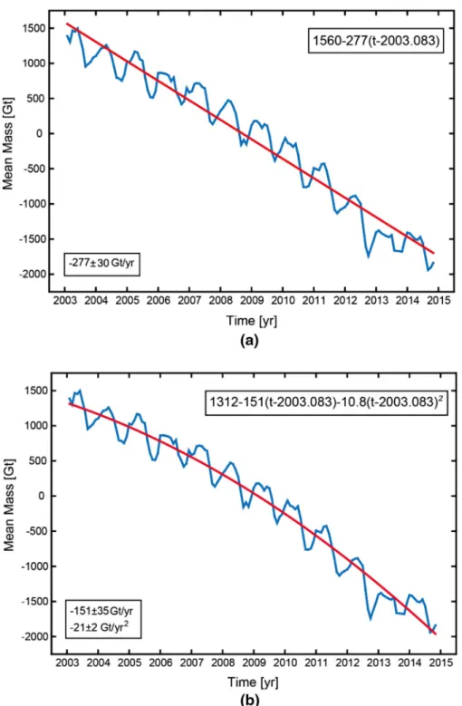
Using Eq. (3) and convolving the GRACE Stokes coefficients with the averaging function of Eq. (4), time series of surface mass variation have been estimated in a 1°91° grid covering Greenland for the period of January 2003–October 2014. We then form an approximate estimate of total mass change for each month by summing the mass change by cosine latitude weighting of the estimates at the different grid elements. Then, linear regression (considering a linear trend, an annual and a semi- annual periodic terms) has been determined for each time-series. Figure1a shows time- series of Greenland monthly mass changes estimated in Gt. We obtain a trend of -277±30 Gt/yr. The uncertainty of 30 Gt/yr is an error estimate and accounts for the least squares adjustment error, the truncation error, the leakage error, the GIA cor- rection and the gravity field model errors. The mass loss is increasing by time from 2003 to 2012 in a relatively consistent pattern, while in the year 2012 a sudden fall of the time series can be observed, which is followed by a relatively less intense melting process (c.f. Fig.1).

In order to determine the acceleration of the mass variation, a quadratic model to the time series has been fitted. The quadratic model includes an acceleration term along with the bias, the linear, the annual and the semiannual terms. For the period 2003–2014, a linear trend of-151±35 Gt/yr and an acceleration of -21±2 Gt/yr² has been deter- mined. The uncertainty of 2 Gt/yr² is an error estimate and accounts for only the least squares adjustment error.

To investigate which of the linear or quadratic models fits better to the time-series, the adjusted R-Squared (RAdj2 ) of the data fit has been determined.RAdj2 is defined as (Johnson and Wichern2002):

R²_Adj¼11R² N1

NM1 ð7Þ

whereR²¼1SSE=SST, where SSE is the sum of squared residuals, SST is the sum of the squared difference of each observation from the mean,Nis the number of observations, andMis the number of term in the model. TheRAdj2 provides a measure of the proportion of variance of the observed signal that can be accounted for by the regression model, adjusting for the number of terms in the model.RAdj2 can take any value less than or equal to 1, with a value closer to 1 indicating a better fit.

Fig. 1 Estimated Greenland monthly mass change from January 2003 to October 2014 from GRACE solutions by CSR processing center. Filtering radius is 250 km. The best fittingalinear andbquadratic trend are shown as red line and curve, respectively

For Greenland, we find that RAdj2 for the quadratic model is 0.988. Comparing the RAdj2

for both models shows that the value for quadratic model is 2% larger than for the linear one, suggesting that the data are better modeled by a quadratic model.

It should be stated here that there are other regression models that can be used, e.g. the moving window least squares fit (Fo¨ldva´ry2012).

Figure1shows that seasonal changes of the ice mass are superimposed on long-period variability. In order to eliminate the long-term trend in Greenland mass variability, the bias, linear trend, annual and semi-annual terms has been subtracted, from which Fig.2a is derived. Similarly, secular acceleration has been determined, c.f. Fig.2b. As seen in Fig.2, largest mass losses are occurring in southern, southeastern and northwestern parts with a maximum of-15 cm/yr and the mass loss is increasing by time in southwestern parts with a maximal acceleration of-2.5 cm/yr².

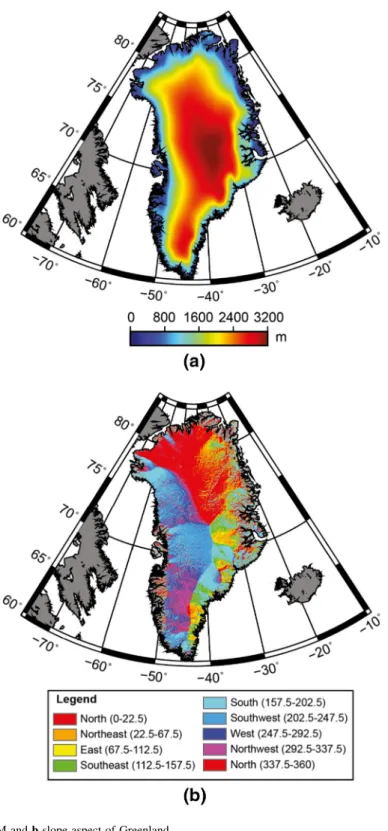
The mass balance is a combination of increased surface temperature, increased snow accumulation, and increased glacial discharge at the coasts. Recent surface mass balance estimates suggest accumulation at high interior elevation and fast melting at low eleva- tions. We test these suggestions by a comparison with the elevations and slope aspects from the Digital Elevation Model (DEM) (GLAS/ICESat 1-km laser altimetry DEM) (DiMarzio et al.2007), c.f. Fig.3. When comparing the DEM (Fig.3a) with the GRACE results of Fig.2a, a relatively inverse relation between ice melting and elevation can be seen. In other words, melting is increased with lower elevation, as expected. In addition, comparing the slope aspect (Fig.3b) with the GRACE results of Fig.2a, ice melting is found to occur mainly on south-facing and west-facing slopes rather than at north-facing and east-facing slopes. It is in accordance with the expectations, since south-facing slopes receive much more heat than the north-facing slopes. In addition, east-facing slopes catch sun only in the morning when temperatures are colder while west-facing slopes catch the sun in the warm afternoon. Consequently, east-facing slopes are colder than west-facing slopes.

The temporal evaluation of Greenland’s mass balance (c.f. Fig.1) shows that mass increases slowly between October and April (e.g. Wouters et al.2008). It also shows mass decrease between May and September. To investigate the mass balance seasonal varia- tions, April–May–June (A–M–J) as months of beginning the melt season, and August–

September–October (A–S–O) as months of ending the melt season are considered. We compute the ‘summer loss’ with subtracting the mass of A–M–J from A–S–O, and the

‘winter gain’ with subtracting the previous year’s A–S–O from the A–M–J. The net of each year is the sum of the summer loss and winter gain of the same year (Joodaki and Nahavandchi2012; Wouters et al.2008).

Table1shows these indicators for each year between 2003 and 2014. The largest net mass loss of -571 Gt was occurred in the year 2012, where we have the maximum summer loss of-733 Gt. In contrast, the year 2013 with the least summer loss of-219 Gt, has the least net mass balance of-5 Gt.

According to Table1, years 2012, 2011, and 2010 had the maximum summer loss, and 2013 and 2006 had the minimum summer loss. As for the winter gains, years 2005, 2011, and 2006 had the maximum, and 2010, 2012, and 2014 had the minimum change.

Fig. 2 GRACE-derived ice mass balancealinear trend andbacceleration in equivalent water thickness forc January 2003–October 2014 over Greenland

Fig. 3 aDEM andbslope aspect of Greenland

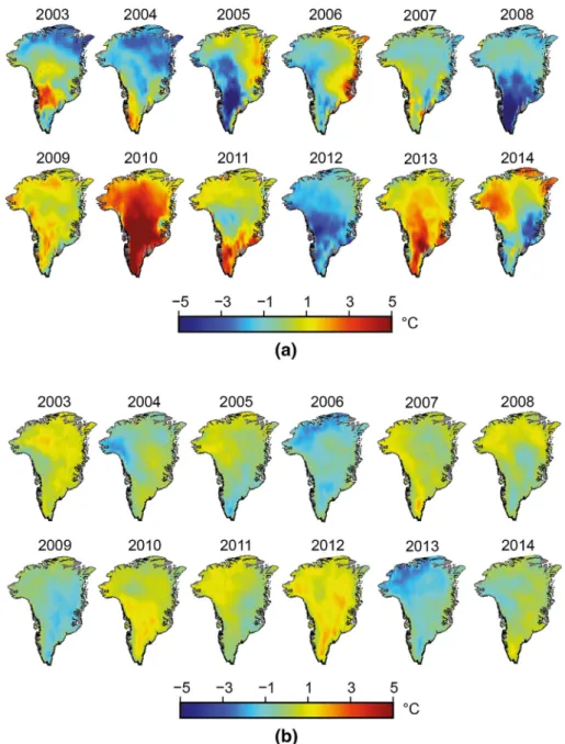
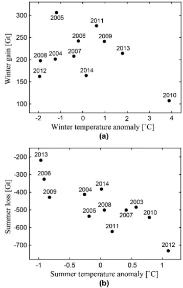
To compare the GRACE results with the temperature changes over Greenland in summer and winter, monthly temperature anomaly with respect to the monthly mean over 2003–2014 period from MODIS-derived IST data has been determined. Figure4shows the mean seasonal anomaly of IST for each year (winter months with respect to the winter mean for period 2003–2014 and summer months with respect to the summer mean for the same period). Comparing the MODIS derived results of Fig.4 with the GRACE derived results of Table1, we find an agreement between summer temperature anomalies and the GRACE-derived summer loss. GRACE-derived mass anomalies show very similar tendency in summer losses and winter gains with the temperature anomaly plots of Fig.4. The comparison also shows that there might be a relative phase difference in time between the ice mass balance derived from GRACE and the seasonal temperature anomalies of MODIS. Figure5 also shows the relationship between mean temperature anomaly and mean winter gain and summer loss. Obviously, in Fig.5 the inverse relationship of temperature anomaly and mass loss is more convincing for the summer period.

In an attempt to study the relationship between the ice mass balance time series and IST time series, continuous wavelet transform (CWT) and the cross wavelet transform (XWT) have been utilized, to expand time-series records into time–frequency space, and to detect common relative phase in time–frequency space. CWT is used to identify the common power in each time-series, while XWT is used to identify relative phase between the time series. These wavelet tools identify localized intermittent periodicities (Toma´s et al.2015).

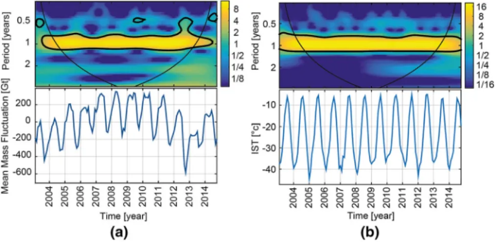
The used Matlab code is provided by the National Oceanography Center (2014). For the wavelet analysis, monthly time series of both ice mass and IST are used. Figure6shows the CWT of both time-series. Note that, the ice mass time series are de-trended. From the analysis of the continuous wavelet power of the ice mass and IST time series, we can observe a clear annual cycle along the whole observation interval for both time series.

Additionally, a semi-annual seasonal fluctuation can be identified along the whole observation period.

The ice surface temperature is a well-known triggering factor of ice melting. To study further the relationship between the ice mass balance and the temperature anomaly, cross

Table 1 Greenland mass bal- ance derived from GRACE monthly gravity field solution provided by CSR between 2003 and 2014

Year A–M–J [Gt]

A–S–O [Gt]

Summer loss [Gt]

Winter gain [Gt]

Net balance [Gt]

2003 1473 988 -485 _ _

2004 1189 777 -412 201 -211

2005 1083 548 -535 306 -229

2006 790 464 -326 242 -84

2007 672 170 -502 208 -294

2008 368 -133 -501 198 -303

2009 108 -322 -430 241 -189

2010 -215 -757 -542 107 -435

2011 -480 -1102 -622 277 -345 2012 -940 -1673 -733 162 -571 2013 -1459 -1678 -219 214 -5 2014 -1514 -1896 -382 164 -218

analysis of the time series was determined. The XWT is equivalent to the complex product of two series. The magnitude of XWT is high only where both CWTs of time- series displays high values simultaneously, so that XWT reveals areas in the two dimensional time–frequency space with high common power. This way time patterns common in the two data sets can be identified. The phase of the XWT indicates the time

Fig. 4 aWinter andbsummer temperature anomaly over Greenland between 2003 and 2014

lag between the two time series. For instance, it is zero when the two time series are coincident in time, and it is ±180° if one is maximum when the other is minimum.

Figure7shows the XWT of ice mass fluctuations and IST in Greenland. A high common power between the two time series in the annual period for the whole study period is evident. Some power signal at the semi-annual period is also evident. The relative phase relationship is shown as arrows, with arrows pointing right if the time lag is zero (in- phase) and pointing left if the time lag is ±180° (anti-phase). The arrows pointing straight down and up indicate ±90° time lag. The XWT analysis shows that ice mass change and ice surface temperature are not in-phase and show anti-phase relationship in all the sectors with significant common power. The results are in agreement with results shown in Table1 and Fig.4.

Fig. 5 Plots ofa winter gain versus winter temperature anomaly and b summer loss versus summer temperature anomaly

4 Conclusion

In this study, mass balance of Greenland ice sheet for January 2003–October 2014 from the GRACE data has been computed. We evaluated the linear and quadratic trends in Greenland at the continental scale. The regions with acceleration signal appears clearly over the area. The mass loss is increasing with time in several regions. Most of Greenland experience this acceleration, with the largest losses in southeastern and northwestern Greenland. In the northwest Greenland, the mass loss is also increasing at a significant level, but its magnitude is lower, and the signal is confined along the coast.

Fig. 6 Continuous wavelet transform ofathe mean mass fluctuation andbIST from 2003 to 2014

Fig. 7 Cross wavelet transform of the ice mass fluctuations and IST.Arrows show the relative phase relationship, in which straight upward arrowsindicate that ice mass changes and IST show anti-phase relationship

Summer loss, winter gain and the net mass balance in Greenland for 2003–2014 have also been evaluated. We found minimum net mass balance in 2012 and 2010 with a maximum in 2013. We found a net mass balance of-571 Gt in 2012, and net mass balance of-5 Gt in 2013. To relate these mass balances to climate effects, we evaluated MODIS- derived seasonal ice surface temperature and compared the temperature profiles with GRACE-derived ice mass changes. The comparison in time domain showed common power between the two data series. To study further, the seasonal relationships between the GRACE and MODIS derived time series, continuous and cross wavelet transforms in time–

frequency domain have been used. Wavelet tool helps to understand the seasonal kinematic behavior of the ice mass fluctuation showing the common power between two time series for the whole study period (2003–2014). We found a high common power between the two time series in annual period for the whole study period. Some power signal at the semi- annual period is also detected. The time series comparison between GRACE ice mass loss and MODIS ice surface temperature has also confirmed that these two data sets are not in- phase.

Acknowledgements This work is a part of a project funded by the Norwegian University of Science and Technology (NTNU). Monthly C20 coefficients from SLR are available athttp://icgem.gfz-potsdam.de.

Degree-1 coefficients and monthly GLDAS and ECCO data are available at http://grace.jpl.nasa.gov.

MODIS-derived IST data are available athttp://modis-snowice.gsfc.nasa.gov/?c=greenland. GLAS/ICESat 1-km laser altimetry DEM are available atftp://sidads.colorado.edu/pub/DATASETS/DEM. The authors would like to thank the editor and two anonymous reviewers for their time and constructive criticism.

References

Baur O, Kuhn M, Featherstone W (2009) GRACE-derived ice-mass variations over Greenland by accounting for leakage effects. J Geophys Res Solid Earth 1978–2012:114. doi:10.1029/2008JB006239 Chen J, Wilson C, Famiglietti J, Rodell M (2005) Spatial sensitivity of the Gravity Recovery and Climate Experiment (GRACE) time-variable gravity observations. J Geophys Res Solid Earth. doi:10.1029/

2004JB003536

Chen J, Wilson C, Tapley B (2006) Satellite gravity measurements confirm accelerated melting of Greenland ice sheet. Science 313:1958–1960. doi:10.1126/science.1129007

DiMarzio J, Brenner A, Schutz R, Shuman C, Zwally H (2007) GLAS/ICESat 1 km laser altimetry digital elevation model of Greenland Digital media. National Snow and Ice Data Center, Boulder Fo¨ldva´ry L (2012) Mass-change acceleration in Antarctica from GRACE monthly gravity field solutions. In:

Geodesy for Planet Earth. Springer, pp 591–596. doi:10.1007/978-3-642-20338-1_72

Fukumori I (2002) A partitioned Kalman filter and smoother. Mon Weather Rev 130:1370–1383. doi:10.

1175/1520-0493(2002)130%3C1370:APKFAS%3E2.0.CO;210.1175/1520-0493(2002)

Geruo A, Wahr J, Zhong S (2013) Computations of the viscoelastic response of a 3-D compressible Earth to surface loading: an application to Glacial Isostatic Adjustment in Antarctica and Canada. Geophys J Int 192:557–572. doi:10.1093/gji/ggs030

Hall DK, Comiso JC, DiGirolamo NE, Shuman CA, Box JE, Koenig LS (2013) Variability in the surface temperature and melt extent of the Greenland ice sheet from MODIS. Geophys Res Lett 40:2114–2120.

doi:10.1002/grl.50240

Houghton JT et al (2001) Climate change 2001: the scientific basis. Contribution of working group I to the third assessment report of the intergovernmental panel on climate change. In. Cambridge University Press, Cambridge, United Kingdom and New York, NY, USA, p 881

Johnson RA, Wichern DW (2002) Applied multivariate statistical analysis, vol 5. Pearson Education, Upper Saddle River

Joodaki G, Nahavandchi H (2012) Mass loss of the Greenland ice sheet from GRACE time-variable gravity measurements. Studia geophysica et geodaetica 56:197–214. doi:10.1007/s11200-010-0091-x Kim S-B, Lee T, Fukumori I (2007) Mechanisms controlling the interannual variation of mixed layer

temperature averaged over the Nin˜o-3 region. J Clim 20:3822–3843. doi:10.1175/JCLI4206.1

National Oceanography Center N (2014) Crosswavelet and wavelet coherence. http://noc.ac.uk/using- science/crosswavelet-wavelet-coherence

Peltier W (2004) Global glacial isostasy and the surface of the ice-age Earth: the ICE-5G (VM2) model and GRACE. Annu Rev Earth Planet Sci 32:111–149. doi:10.1146/annurev.earth.32.082503.144359 Ramillien G, Lombard A, Cazenave A, Ivins E, Llubes M, Remy F, Biancale R (2006) Interannual variations

of the mass balance of the Antarctica and Greenland ice sheets from GRACE. Global Planet Change 53:198–208. doi:10.1016/j.gloplacha.2006.06.003

Rodell M et al (2004) The global land data assimilation system. Bull Am Meteorol Soc 85:381–394. doi:10.

1175/BAMS-85-3-381

Sørensen LS et al (2011) Mass balance of the Greenland ice sheet (2003–2008) from ICESat data–the impact of interpolation, sampling and firn density. Cryosphere 5:173–186. doi:10.5194/tc-5-173-2011 Slobbe D, Ditmar P, Lindenbergh R (2009) Estimating the rates of mass change, ice volume change and

snow volume change in Greenland from ICESat and GRACE data. Geophys J Int 176:95–106. doi:10.

1111/j.1365-246X.2008.03978.x

Sos´nica K, Ja¨ggi A, Thaller D, Beutler G, Dach R (2014) Contribution of Starlette, Stella, and AJISAI to the SLR-derived global reference frame. J Geod 88:789–804. doi:10.1007/s00190-014-0722-z

Swenson S, Wahr J (2006) Post-processing removal of correlated errors in GRACE data. Geophys Res Lett.

doi:10.1029/2005GL025285

Swenson S, Wahr J, Milly P (2003) Estimated accuracies of regional water storage variations inferred from the Gravity Recovery and Climate Experiment (GRACE). Water Resour Res. doi:10.1029/

2002WR001808

Swenson S, Chambers D, Wahr J (2008) Estimating geocenter variations from a combination of GRACE and ocean model output. J Geophys Res Solid Earth. doi:10.1029/2007JB005338

Tapley BD, Bettadpur S, Ries JC, Thompson PF, Watkins MM (2004) GRACE measurements of mass variability in the Earth system. Science 305:503–505. doi:10.1126/science.1099192

Toma´s R, Li Z, Lopez-Sanchez J, Liu P, Singleton A (2015) Using wavelet tools to analyse seasonal variations from InSAR time-series data: a case study of the Huangtupo landslide. Landslides. doi:10.

1007/s10346-015-0589-y

Velicogna I, Wahr J (2005) Greenland mass balance from GRACE. Geophys Res Lett. doi:10.1029/

2005GL023955

Velicogna I, Wahr J (2006) Acceleration of Greenland ice mass loss in spring 2004. Nature 443:329–331.

doi:10.1038/nature05168

Velicogna I, Wahr J (2013) Time-variable gravity observations of ice sheet mass balance: precision and limitations of the GRACE satellite data. Geophys Res Lett 40:3055–3063. doi:10.1002/grl.50527 Velicogna I, Sutterley T, van den Broeke M (2014) Regional acceleration in ice mass loss from Greenland

and Antarctica using GRACE time-variable gravity data. Geophys Res Lett 41:8130–8137. doi:10.

1002/2014GL061052

Wahr J, Molenaar M, Bryan F (1998) Time variability of the Earth’s gravity field: hydrological and oceanic effects and their possible detection using GRACE. J Geophys Res Solid Earth (1978–2012) 103:30205–30229. doi:10.1029/98JB02844

Wouters B, Chambers D, Schrama E (2008) GRACE observes small-scale mass loss in Greenland. Geophys Res Lett. doi:10.1029/2008GL034816