Recent Increases in Winter Snowfall Provide Resilience to Very Small Glaciers in the Julian Alps, Europe

(1)

atmosphere

Article

Recent Increases in Winter Snowfall Provide Resilience to Very Small Glaciers in the Julian Alps, Europe

Renato R. Colucci^1,2,*^,† , Manja Žebre^3,‡, Csaba Zsolt Torma⁴ , Neil F. Glasser³ , Eleonora Maset⁵ , Costanza Del Gobbo^2,6and Simone Pillon²

Citation: Colucci, R.R.; Žebre, M.;

Torma, C.Z.; Glasser, N.F.; Maset, E.;

Del Gobbo, C.; Pillon, S. Recent Increases in Winter Snowfall Provide Resilience to Very Small Glaciers in the Julian Alps, Europe.Atmosphere 2021,12, 263. https://doi.org/

10.3390/atmos12020263

Academic Editor: Scott Osprey

Received: 26 November 2020 Accepted: 9 February 2021 Published: 17 February 2021

Publisher’s Note:MDPI stays neutral with regard to jurisdictional claims in published maps and institutional affil- iations.

Licensee MDPI, Basel, Switzerland.

This article is an open access article distributed under the terms and conditions of the Creative Commons Attribution (CC BY) license (https://

creativecommons.org/licenses/by/

4.0/).

1 CNR—Institute of Polar Sciences c/o Scientific Campus Ca’ Foscari University in Venice, 30172 Mestre (VE), Italy

2 Department of Mathematics and Geosciences, University of Trieste, 34100 Trieste, Italy;

costanza.delgobbo@gmail.com (C.D.G.); pillon.simone@gmail.com (S.P.)

3 Department of Geography & Earth Sciences, Aberystwyth University, Aberystwyth SY23 3FL, UK;

Manja.Zebre@geo-zs.si (M.Ž.); nfg@aber.ac.uk (N.F.G.)

4 Department of Meteorology, Eötvös Loránd University, 1117 Budapest, Hungary; tcsabi@caesar.elte.hu

5 Polytechnic Department of Engineering and Architecture, University of Udine, 33100 Udine, Italy;

eleonora.maset.1@gmail.com

6 International Centre for Theoretical Physics, 34151 Trieste, Italy

* Correspondence: renato.colucci@isp.cnr.it

† Previously at CNR-ISMAR Trieste, Italy.

‡ Currently at Geological Survey of Slovenia, Ljubljana, Slovenia.

Abstract:Very small glaciers (<0.5 km²) account for more than 80% of the total number of glaciers and more than 15% of the total glacier area in the European Alps. This study seeks to better understand the impact of extreme snowfall events on the resilience of very small glaciers and ice patches in the southeastern European Alps, an area with the highest mean annual precipitation in the entire Alpine chain. Mean annual precipitation here is up to 3300 mm water equivalent, and the winter snow accumulation is approximately 6.80 m at 1800 m asl averaged over the period 1979–2018. As a consequence, very small glaciers and ice/firn patches are still present in this area at rather low altitudes (1830–2340 m). We performed repeated geodetic mass balance measurements on 14 ice bodies during the period 2006–2018 and the results show an increase greater than 10% increase in ice volume over this period. This is in accordance with several extreme winter snow accumulations in the 2000s, promoting a positive mass balance in the following years. The long-term evolution of these very small glaciers and ice bodies matches well with changes in mean temperature of the ablation season linked to variability of Atlantic Multidecadal Oscillation. Nevertheless, the recent behaviour of such residual ice masses in this area where orographic precipitation represents an important component of weather amplification is somehow different to most of the Alps. We analysed synoptic meteorological conditions leading to the exceptional snowy winters in the 2000s, which appear to be related to the influence and modification of atmospheric planetary waves and Arctic Amplification, with further positive feedbacks due to change in local sea surface temperature and its interactions with low level flows and the orography. Although further summer warming is expected in the next decades, we conclude that modification of storm tracks and more frequent occurrence of extreme snowfall events during winter are crucial in ensuring the resilience of small glacial remnants in maritime alpine sectors.

Keywords:small glaciers; glacier mass balance; climate; AMO; precipitation; climate change

1. Introduction

Ice bodies in the Julian Alps are typically in the smallest size category of glaciers, with several glacial and nival ice patches [1] and one small mountain glacier [2]. These very small ice masses have gained an increasing scientific importance in the last few decades e.g., in the studies of Mediterranean [3] glaciation during the Pleistocene and the Holocene [4]

Atmosphere2021,12, 263. https://doi.org/10.3390/atmos12020263 https://www.mdpi.com/journal/atmosphere

(2)

Atmosphere2021,12, 263 2 of 25

and elsewhere. Small glaciers represent relevant component of the cryosphere contributing to landscape formation, local hydrology and sea level-rise [3]. At a regional scale like the European Alps, residual ice masses may occupy a significant volume fraction and their omission could result in errors of±10%. For this reason, several authors stressed to the production of accurate inventories considering all ice bodies down to 0.01 km²or smaller in order to reduce uncertainties [5,6]. Despite their small size, they are widespread and likely account for about 80–90% of the total number of mid- to low-latitude ice bodies in mountain ranges. For this reason, it is important to understand their behaviour [7].

The Alpine landscape is rapidly changing due to global warming and larger ice masses continue to disintegrate into smaller ice bodies (e.g., [2,8–10]). In the future, alpine glaciers will be likely characterized by a larger number of these very small ice bodies, especially in karstic terrains. Indeed, the cryosphere is rapidly declining in most, if not all, high elevation environments on Earth [11] and anthropogenic climate change is thought to be the main cause in accelerating this process over the next few decades. In the European Alps a rapid glacier retreat and downwasting has been observed in the early 21st century with regionally variable ice thickness changes of−0.5 to−0.9ma⁻¹and an estimated 2000–2014 mass loss of 1.3±0.2 Gt a⁻¹[12]. The Equilibrium Line Altitude (ELA) in the Alps rose by 170–250 m in the last few decades [13], and in the Julian Alps, the Environmental ELA (envELA; [14]), the temperature-precipitation-dependent ELA [15,16], rose from 2350 to 2750 m between the early 1980s to the beginning of the 2000s [17]. The main cause for glacier retreat in the Alps is related to longer and warmer summers modulated by winter precipitation anomalies [11,13,18–20]). Nevertheless, the magnitude of these impacts is both site- and catchment-specific and depends on the resilience and buffering capacities of the system, including the area occupied by glaciers and permafrost, basin hypsometry, groundwater systems, vegetation type and cover, and ecosystem types [21–23]. Such ongoing major and unprecedented glacier decline strongly affects also the integrity and value of several World Heritage sites [20].

Very small glaciers are very sensitive to climatic change and subsequently their areas may change significantly on a decadal, and even on a yearly basis [24]. Nevertheless, small glaciers and ice patches in some sectors of the Alps as well as in some Mediterranean areas have surprisingly shown a slowdown in the reduction rate from the mid-2000s even though summer temperatures continued to rise at double the rate of the global average [2,17,25–30]. This is especially true in more maritime environments where mean annual precipitation (MAP) is very high or where the topography favours snow accumulation [31–33] Based on high-resolution and high quality daily precipitation measurements, the Julian Alps is considered as a mesoscale hot spot of heavy precipitation [34] where the highest alpine MAP is recorded [35]. Furthermore, total precipitation has different origins over the northern and southern flanks of the chain: precipitation is more frequent but with lower intensity to the north, while much of the total precipitation to the south is due to rare intense weather events [34]. Local feedbacks and synoptic conditions can favour or even moderate such events.

Variation in the large-scale atmospheric circulation, in part associated with climatic modes of variability such as the North Atlantic Oscillation (NAO) and the Atlantic Multi- decadal Oscillation (AMO), produces different synoptic conditions (Northern Hemisphere teleconnection patterns, cyclones) leading to a high interannual variability of temperature and winter precipitation over the Alps [36,37].

NAO is an irregular fluctuation of surface atmospheric pressure over the North Atlantic Ocean involving the subtropical high located over the Azores islands and the semi- permanent subpolar low pressure system centered over Iceland [38]. In wintertime the NAO can be considered as the most energetic mode of climate variability in the northern hemisphere that can also manifest itself in extreme weather events [39].

AMO explains multidecadal sea surface temperature (SST) variability in the North Atlantic Ocean from 0^◦ to 70^◦N, with a cycle of 65–70 years and 0.4^◦C range between extremes [40]. Accordingly, as one of the most prominent modes of climate variability,

(3)

AMO also influences Europe’s climate [41]. For instance, it has already proven that AMO has impact on severe cold events across Europe as the positive phase of the AMO manifests in more frequent negative NAO, thus more blocking events associated with extreme weather conditions might occur [42]. The primary influence of AMO on alpine climate is on mean air temperature, while its influence on precipitation is less clear [43,44].

Precipitation, both in winter and summer, is strongly influenced by the position of blocking high [45]. Long-lasting high pressure system, which blocks the moisture air or Atlantic winter cyclones penetrating from the west, leads to stable conditions along with the downwelling motions [46]. Accordingly, during wintertime within a region where weather conditions are dominated by an anticyclone, over the basins surrounded by mountains, sharp temperature inversion can occur [47,48]. Furthermore, It has also been recognized already in the late 19th century that specific cyclone tracks can lead to abundant large-scale precipitation and even snowstorms in the region of central Europe [49]. It is also interesting to note that van Bebber’s type cyclones (Vb, fifth subcategory of cyclone that follows van Bebber’s track, [49]), which move from the east-southeast of Europe into the inner part of Europe can be related to heavy precipitation (95th percentile) events. These relatively rare events can be associated with heavy precipitation manifested over the northern slopes of the Alps.

The aims of this paper are (1) to report mass balance observations over the period 2006–2018 for very small glaciers in the Italian part of the Julian Alps (southeastern Eu- ropean Alps) obtained from multiannual geodetic surveys performed by using LiDAR techniques, theodolite measurements and GIS analysis; (2) to link the change in mass balance with associated weather patterns and their possible local amplifications, with a focus on extreme snowy winters observed over the same time span.

2. Study Area

The Julian Alps, designated in 2019 from UNESCO (United Nations Educational, Scien- tific and Cultural Organization) as a Biosphere Reserve (https://en.unesco.org/biosphere/

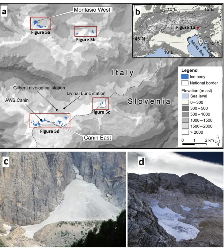
eu-na/julian-alps-italy; last accessed 15 July 2020), occupy 1853 km², spanning west to east across the Italian–Slovenian border (Figure1). The mountain range is characterized by Upper Triassic carbonate succession of dolostone (Dolomia Principale) and limestone (Dachstein limestone), and glaciokarst landscape [50] is widespread. The drainage divide between the Adriatic Sea and the Black Sea crosses Julian Alps in the range of Mount Canin-Kanin (2587 m asl; Figure1), which represents an important groundwater storage in the area [51,52]. Mount Montasio (2754 m asl) is the highest peak in the Italian side of the Julian Alps. The area is recognized as the wettest in the Alps with quite constant precipitation contributions from all seasons [35]. The 1981–2010 climatology of the Mt.

Canin-Kanin area has been reconstructed by [28] at an elevation of 2200 m asl (AWS Canin, Figure1a). MAP is estimated at 3335 mm water equivalent (w.e.) with February the driest month (180 mm w.e.) and November the wettest (460 mm w.e.). Mean annual air temperature (MAAT) is 1.1±0.6^◦C. February is the coldest month (−6.0±2.9^◦C) and July the warmest (9.2±1.3^◦C).

Average winter snow accumulation of 6.80 m was measured between December and April from 1972–2018 at 1830 m a.s.l. at the Gilberti nivological station (Figure1a).

Snow thickness on the ground is also recorded at Livinal Lunc weathter station (Figure1a).

The present mean envELA is estimated at about 2700 m asl [17], which means it is at present located above the highest peaks except for Mount Montasio. From the end of the little ice age (LIA; about AD 1865), glaciers in the Julian Alps have retreated significantly, and the majority changed in status from glaciers to either small glaciers, very small glaciers, ice patches of glacial origin [1], buried ice patches (permafrost patches), or simply no ice at all [17,31]. Since the LIA peak in ice extent, the volume decreased by about 96%. In 2012, 19 very small ice bodies still existed in the study area, having areas from 2·10⁻³km²to 71·10⁻³km²and estimated volumes from 0.002·10⁻³km³to 0.822·10⁻³km³[31]. The only ice body retaining the characteristics of a mountain glacier is the Montasio West, while the

(4)

Canin East is an ice patch of glacial origin or Glacier Ice Patch (GIP; Figure1). In 2011 this GIP had a volume of 205,000 m³, an area of 17,530 m², and a mean thickness of 11.7 m [53].

Atmosphere 2021, 12, x FOR PEER REVIEW 4 of 26

Figure 1. (a) Distribution of ice bodies in the Italian Julian Alps. (b) Location of the Julian Alps study area. (c) Montasio West glacier. (d) Canin East glacier ice patch. Photo R.R. Colucci.

Average winter snow accumulation of 6.80 m was measured between December and April from 1972–2018 at 1830 m a.s.l. at the Gilberti nivological station (Figure 1a). Snow thickness on the ground is also recorded at Livinal Lunc weathter station (Figure 1a). The present mean envELA is estimated at about 2700 m asl [17], which means it is at present located above the highest peaks except for Mount Montasio. From the end of the little ice age (LIA; about AD 1865), glaciers in the Julian Alps have retreated significantly, and the majority changed in status from glaciers to either small glaciers, very small glaciers, ice patches of glacial origin [1], buried ice patches (permafrost patches), or simply no ice at Figure 1.(a) Distribution of ice bodies in the Italian Julian Alps. (b) Location of the Julian Alps study area. (c) Montasio West glacier. (d) Canin East glacier ice patch. Photo R.R. Colucci.

3. Data and Methods

3.1. Topography-Related Glacier Data and Analysis

We used different geospatial data, such as LiDAR, theodolite-generated ground control points (GCPs) and digital orthophotos dated to the period 2006–2018 in order to derive

(5)

outlines of all ice bodies in the Italian sector of the Julian Alps (n = 33) and calculate their surface elevation change and volume change during this period. We also calculated annual and 12-year cumulative geodetic mass balance of the Canin East GIP for the period 2006–2018. This GIP was chosen as a case study for the annual mass balance measurements because there is a long historic record of its front variations [17] and recently acquired internal structure and densities of different units within this ice body [53]. We used ESRI ArcGIS^® and the WGS1984 UTM Zone 33N spatial reference system for mapping and analyzing the geospatial data.

3.2. LiDAR Data Acquisition and Processing

Airborne LiDAR (Light Detection and Ranging) data were acquired over the study area in the years 2006, 2011, 2013, 2015, 2016 and 2018, with an average point density greater than 4 points per square meter. All the surveys were carried out in the same period of the year, between 13 September and 1 October. Technical specifications of the data acquisition process are reported in Table1. The point clouds were then exploited to create Digital Elevation Models (DEMs) with a resolution of 1 m. In particular, the software employed for this task, TerraScan by TerraSolid, uses LiDAR points to derive a Triangulated Irregular Network (TIN) through Delaunay triangulation that is subsequently resampled onto a grid of specified resolution.

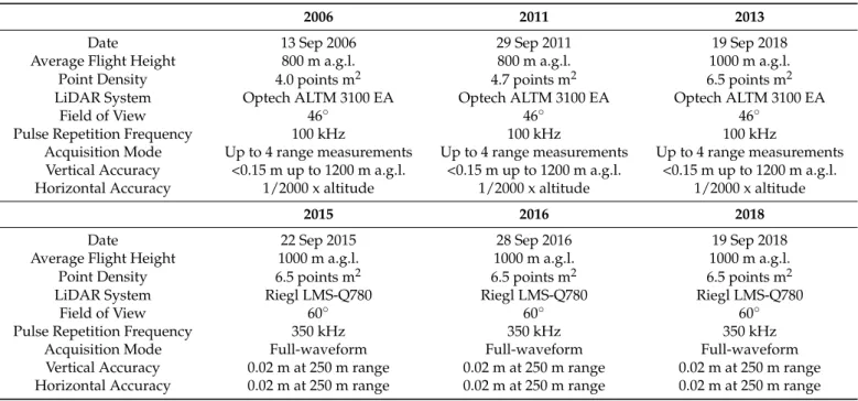
Table 1.Technical specifications of the LiDAR surveys performed in the study area between 2006 and 2018.

2006 2011 2013

Date 13 Sep 2006 29 Sep 2011 19 Sep 2018

Average Flight Height 800 m a.g.l. 800 m a.g.l. 1000 m a.g.l.

Point Density 4.0 points m² 4.7 points m² 6.5 points m²

LiDAR System Optech ALTM 3100 EA Optech ALTM 3100 EA Optech ALTM 3100 EA

Field of View 46^◦ 46^◦ 46^◦

Pulse Repetition Frequency 100 kHz 100 kHz 100 kHz

Acquisition Mode Up to 4 range measurements Up to 4 range measurements Up to 4 range measurements Vertical Accuracy <0.15 m up to 1200 m a.g.l. <0.15 m up to 1200 m a.g.l. <0.15 m up to 1200 m a.g.l.

Horizontal Accuracy 1/2000 x altitude 1/2000 x altitude 1/2000 x altitude

2015 2016 2018

Date 22 Sep 2015 28 Sep 2016 19 Sep 2018

Average Flight Height 1000 m a.g.l. 1000 m a.g.l. 1000 m a.g.l.

Point Density 6.5 points m² 6.5 points m² 6.5 points m²

LiDAR System Riegl LMS-Q780 Riegl LMS-Q780 Riegl LMS-Q780

Field of View 60^◦ 60^◦ 60^◦

Pulse Repetition Frequency 350 kHz 350 kHz 350 kHz

Acquisition Mode Full-waveform Full-waveform Full-waveform

Vertical Accuracy 0.02 m at 250 m range 0.02 m at 250 m range 0.02 m at 250 m range Horizontal Accuracy 0.02 m at 250 m range 0.02 m at 250 m range 0.02 m at 250 m range

3.3. Theodolite-Generated Ground Control Points (GCPs)

Manual field surveys were performed using a total station instead of GPS due to no or patchy network real time kinematic (NRTK) available correction and the difficulty of obtaining a sufficient number of satellites. To do this, five ground control points (GCPs) were previously located in the vicinity of the GIP to assure repeatable measurements with a total station. The total station was a Stonex R9 DR1000 robotic. One of the GCPs is located just on the Canin automatic weather station (AWS) that ensures good visibility even in case of large amount of snow on the ground. Points on the GIP were surveyed using a pole-mounted 360^◦prism. The furthest surveyed point is about 300 m from the GCP, and with this configuration, the accuracy of the survey is centimetric.

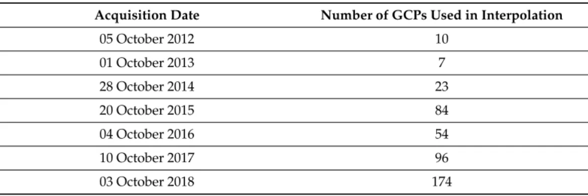
GCPs (Table2) were exploited to create digital elevation models (DEMs) with a resolution of 1 m for every year between 2012 and 2018. Different interpolation methods,

(6)

such as natural neighbour, spline, inverse distance weighted and topo to raster, were tested to derive DEMs from GCPs. We computed a DEM of Difference (DoD) by subtracting the LiDAR derived DEM from GCPs-derived DEM for the years 2013, 2015, 2016 and 2018, when both LiDAR and theodolite generated GCPs data were available. Average elevation difference and standard deviation were computed for every DoD. Both natural neighbour and spline interpolation methods gave on average the smallest average elevation difference (0.26 m) between the LiDAR derived and GCPs-derived DEMs (Table3). Moreover, natural neighbor interpolation method gave on average the lowest standard deviation (0.36 m).

Therefore, GCPs-derived DEMs for years 2012, 2014 and 2017, for which there is no LiDAR data available, were generated using natural neighbour interpolation method and used for further GIP-related computations. For years when both theodolite-generated GCPs and LiDAR data are available, we favour the LiDAR derived DEMs for GIP surface elevation change calculations due to higher point density and consequently higher accuracy of DEM.

GCPs served also for quantifying ice-body dynamics for the period 2012–2017.

Table 2.Acquisition date and number of theodolite-generated ground control points (GCPs).

Acquisition Date Number of GCPs Used in Interpolation

05 October 2012 10

01 October 2013 7

28 October 2014 23

20 October 2015 84

04 October 2016 54

10 October 2017 96

03 October 2018 174

Table 3.Average elevation difference (in meters) of the Canin East Glacier Ice Patch (GIP) digital elevation model (DEM) of Difference (DoD) between LiDAR derived DEM through Delaunay triangulation and GCPs-derived DEM using natural neighbor, spline, inverse distance weighted and topo to raster interpolation methods.

Year

Time Difference (in days) between

LiDAR and GCP Surveys

LIDAR DEM—GCP DEM Natural Neighbour

LiDAR DEM—GCP DEM Spline

LiDAR DEM—GCP DEM Inverse Distance Weighted

LiDAR DEM—GCP DEM Topo to Raster

2013 0 −0.44 −0.09 −1.01 −0.28

2015 28 0.19 0.39 0.05 0.27

2016 6 −0.08 0.13 −0.18 0.24

2018 14 0.33 0.44 0.14 0.42

Average of Absolute

Values 0.26 0.26 0.35 0.3

3.4. Ice Body Measurements

We manually digitised the surface area of all the glaciers and ice patches in the Italian Julian Alps for the years 2006 and 2018 with the use of digital orthophotos and 1 m resolution LiDAR-derived shaded relief. The associated absolute error by using this method, according to Fitzharris et al. (1997) [54] is about±25 m². Abermann et al. 2010 for glaciers smaller than 1 km²(which is 2 orders of magnitude larger than our ice bodies) indicate a larger error of±5%. The surface area of the Canin East GIP was mapped for the year 2006 and for every year between 2011 and 2018 using digital orthophotos, 1 m resolution LiDAR derived shaded relief or theodolite-generated GCPs taken at the GIP margin (Figure2).

Each DEM was clipped by the corresponding GIP area so that all cells in the DEM represent snow-, firn-, and ice-covered areas. We then computed a DoD of sequential DEMs by subtracting DEM at a later time from a DEM at an earlier time in order to obtain the surface elevation change of the Canin East GIP for every year between 2011–2018, a 5-year

(7)

period between 2006–2011 and a 12-year period between 2006–2018. For the rest of the ice bodies in the Italian Julian Alps, we only computed DoD for the 12-year period 2006–2018.

Average surface elevation change of each DoD was then multiplied with the corresponding surface area, which yielded a volume change.

using a floating-date systems [56], where the surveys were carried out close to the end of the ablation period (see Tables 1 and 2).

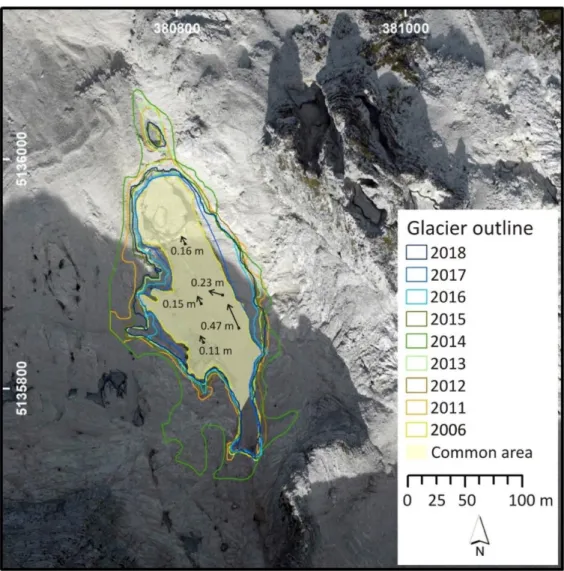
Figure 2. Outlines of the Canin East GIP for the period 2006–2018. Common area, which was used for surface elevation changes and further in mass balance calculations, represents the intersect area from all observational years in the period 2006–2018. Black arrows show glacier movement in the 5-year-period 2012–2017; note they are not in scale with the map but elongated for clarity. Base layer is 2006 digital orthophoto.

3.5. Climate Data and Analysis 3.5.1. ERA Interim Dataset

The meteorological variables (wind fields at 10 m above surface, sea level pressure, precipitation) used in this study in order to analyse synoptic conditions are provided by the ERA-Interim dataset [57]. The ERA-Interim is an atmospheric reanalysis dataset produced by the European Centre for Medium-Range Weather Forecasts (ECMWF) for the whole globe. The data assimilation system used to produce ERA-Interim includes a 4- dimensional variational analysis (4D-Var) technique with a 12-h analysis window. Addi- tionally, the ERA-Interim dataset is freely available for the period 01.01.1979–31.08.2019 (noting that the ERA-Interim dataset has been superseded by the ERA5 dataset, [58]) at approximately 80 km grid resolution and on 60 vertical levels from surface to 0.1 hPa, which makes this dataset ideal for analysing synoptic situations leading to abundant precipitation or long-lasting rainless events over a specific region in Europe. Figure S1 reports Figure 2.Outlines of the Canin East GIP for the period 2006–2018. Common area, which was used for surface elevation changes and further in mass balance calculations, represents the intersect area from all observational years in the period 2006–2018. Black arrows show glacier movement in the 5-year-period 2012–2017; note they are not in scale with the map but elongated for clarity. Base layer is 2006 digital orthophoto.

Unlike the volume change calculations, where the yearly area change was fully taken into account, we used a common area to compute the geodetic mass balance of the Canin East GIP. The common area is the intersect area from all observational years in the period 2006–2018 and, moreover, does not include the uppermost part of the GIP that is mainly debris-covered (Figure2). Thus, the common area is the most stable area of the GIP and therefore the most appropriate for the mass balance calculations. Geodetic mass balance was computed by multiplying average surface elevation change with the density of the GIP material. The density of this ice body was previously estimated to 791 kg m⁻³ by [53] using ground penetrating radar in 2011, and this value was applied to compute the geodetic mass balance. Due to larger quantities of residual winter snow/firn in years 2013–2015 and 2018, a density of 650 kg m⁻³was used in mass balance calculations for these years [53–55]. Annual geodetic mass balance was calculated between 2011 and 2018, while a 5-year (2006–2011) and a 12-year (2006–2018) cumulative geodetic mass balances

(8)

were also obtained. The latter was calculated also for all other ice bodies in the Italian Julian Alps using the intersect area, and the conversion factor of 791 kg m⁻³was applied as in the case of the Canin East GIP. We determined the mass balance year for balance calculations using a floating-date systems [56], where the surveys were carried out close to the end of the ablation period (see Tables1and2).

3.5. Climate Data and Analysis 3.5.1. ERA Interim Dataset

The meteorological variables (wind fields at 10 m above surface, sea level pressure, precipitation) used in this study in order to analyse synoptic conditions are provided by the ERA-Interim dataset [57]. The ERA-Interim is an atmospheric reanalysis dataset produced by the European Centre for Medium-Range Weather Forecasts (ECMWF) for the whole globe. The data assimilation system used to produce ERA-Interim includes a 4-dimensional variational analysis (4D-Var) technique with a 12-h analysis window. Additionally, the ERA- Interim dataset is freely available for the period 01.01.1979–31.08.2019 (noting that the ERA- Interim dataset has been superseded by the ERA5 dataset, [58]) at approximately 80 km grid resolution and on 60 vertical levels from surface to 0.1 hPa, which makes this dataset ideal for analysing synoptic situations leading to abundant precipitation or long-lasting rainless events over a specific region in Europe. Figure S1 reports the differences between the aforementioned datasets for winter periods with low- and high snow accumulation.

3.5.2. NAO and AMO Index Data

The North Atlantic Oscillation (NAO) index data and the Atlantic Multidecadal Os- cillation (AMO) index data were provided by the National Oceanic and Atmospheric Administration (NOAA). The period between January 1950 and December 2000 for the NAO and 1856 to present for the AMO served as reference for the calculations. Daily and monthly mean NAO index is freely available via NOAA. In this study, we used data based on daily and monthly information. The NAO teleconnection index is obtained through a procedure (Rotated Principal Component Analysis; Barnston and Livezey, 1987), which iso- lates the primary teleconnection patterns, and is applied to the monthly standardized 500 mb height anomalies over the region embedded between 20^◦N-90^◦N.

3.5.3. Local Temperature, Precipitation and Glacier Length

Mean summer air temperature (MSAT) and winter precipitation data come from [28]

and are updated for the last 6 years from meteorological data recorded at the Canin AWS (Figure1) located at an elevation of 2203 m. Snow thickness has been measured since 1972 at the nivological station of Gilberti (Figure1) at an altitude of 1830 m a.s.l.

(source Regional Administration of Friuli Venezia Giulia, snow and avalanches officehttp:

//www.regione.fvg.it/asp/valanghe/welcome.asp; last accessed 5 August 2020). Data on glacier length come from the Italian Glaciological Committee reports [59]. The sum of melting during the ablation season is computed by using a temperature index, i.e., a degree- day model which is one of the most widely used methods for hydrological and ice-dynamic modelling as well as climate sensitivity studies [47,60]. Although simple, this method is a powerful tool, at times even more reliable than energy balance models at a catchment scale [61]. The amount of melting in mm w.e was calculated by applying a Positive degree- day model with a degree-day factor for melting snow of 4.0 cm day⁻¹K⁻¹[47,60,61].

4. Results 4.1. Glacier Area

The area of the Canin East GIP varied substantially over the 12-year observational period (2006–2018) without any decreasing trend (Table4). The largest area (27,448 m²) was observed in 2014, which was more than twice (243%) the area of 2006, when the GIP was the smallest in size. The GIP reached the second largest area (19,425 m²) in 2011, with increase of 72% with respect to 2006. The annual areal changes are more or less equivalent around

(9)

the entire GIP’s edge. The GIP commonly constitutes a continuous ice body but has a smaller area at the terminus, which tends to separate from the main ice body during negative mass balance years. The area of the Canin East GIP in 2018 was equal to 15,914 m², which represents 41% increase in area with respect to 2006 (11,310 m²). The area of Montasio West glacier over the same period did not show significant variations, showing just a very small, 0.05% decrease from 2006 (66,096 m^2.) to 2018 (65,724 m²). The increase in area in 2018 (294,640 m²) with respect to 2006 (240,053 m²) was equal to 18.5% for all the ice patches in the Italian Julian Alps (Supplementary Table S1). It is important to note how large fluctuations in ice patch areas are strictly dependent on residual snow andfirnof the previous winter(s). Both surveys were performed at the end of the ablation season with no fresh snow on the ground that could have affected the accuracy of data.

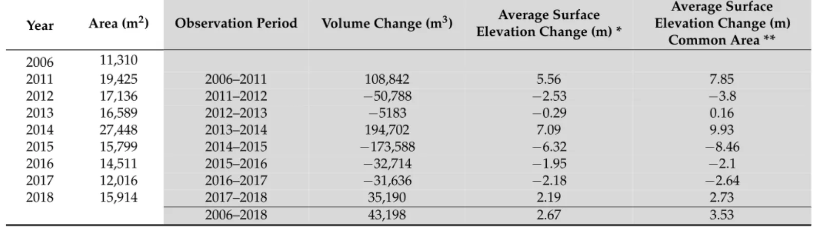
Table 4.Area, volume change and average surface elevation change of the Canin east GIP for the period 2006–2018. Areas of the ice patch at the end of the ablation season are showed in the left (White) part of the Table (First 2 columns from Left).

Average surface elevation changes are reported both for the union of glacier areas at the beginning and at the end of the respective observation periods (*) and for the common area (**) on the right (Grey) side of the Table. The later data was used for the mass balance calculations, whereas the first for the volume change calculations.

Year Area (m²) Observation Period Volume Change (m³) Average Surface Elevation Change (m) *

Average Surface Elevation Change (m)

Common Area **

2006 11,310

2011 19,425 2006–2011 108,842 5.56 7.85

2012 17,136 2011–2012 −50,788 −2.53 −3.8

2013 16,589 2012–2013 −5183 −0.29 0.16

2014 27,448 2013–2014 194,702 7.09 9.93

2015 15,799 2014–2015 −173,588 −6.32 −8.46

2016 14,511 2015–2016 −32,714 −1.95 −2.1

2017 12,016 2016–2017 −31,636 −2.18 −2.64

2018 15,914 2017–2018 35,190 2.19 2.73

2006–2018 43,198 2.67 3.53

4.2. Geodetic Mass Balance and Volume Change

The five-year cumulative mass balance of the Canin East GIP was strongly positive with 6.21 m w.e. between 2006 and 2011 (Figures3and4). Annual mass balances between 2012 and 2018 varied considerably. Annual mass balances in 2012, 2015–2017 were negative with 2015 having the lowest mass balance on record at −5.50 m w.e.

(Figures3and4). In 2014, the GIP experienced its most strongly positive year with mass balance of 6.46 m w.e., when all its surface was still abundantly covered with snow from the previous winter at the end of the ablation season. The year 2018 was the second most positive year at 1.77 m w.e. In 2013, the mass balance was almost neutral but still positive at 0.11 m w.e. Cumulatively, the GIP gained 2.79 m w.e. between 2006 and 2018, although the last 7-year cumulative mass balance was negative (−3.42 m w.e.) (Figures3–5). A 12- year (2006–2018) mean cumulative mass balance of all 33 ice bodies in the Italian Julian Alps was positive too with 2.04 m w.e. (Figure5, Table S1). All ice bodies experienced positive mass balance, with Carnizza-Riofreddo-Studence sector (Figure5b) having the lowest mass balance (0.50 m w.e.) and Cergnala sector (Figure5c) with the highest mass balance (2.66 m w.e.) The Canin sector (Figure5d) experienced the second most positive mass balance (2.22 m w.e.) among all sectors and 0.34 m w.e. lower mass balance from the Canin East GIP. The Montasio West glacier recorded a positive mass balance of 0.13 m w.e.

(Figure5a)

(10)

AtmosphereAtmosphere 2021, 12, x FOR PEER REVIEW 2021,12, 263 10 of 2511 of 26

Figure 3. (a) Annual and cumulated geodetic mass balance of the Canin East GIP (Y_canin and Cum_canin) based on a common area (see Figure 2 for details) compared to 2000–2018 WGMS annual and cumulated mass balance in the Alps (Y_wgms and Cum_wgms) and 2000–2016 optical satellite images annual mass balance calculation based on SLA-METHOD [15] (Y_davaze and cum_davaze)[19]; (b) 11 years (left) and 13 years (right) cumulative mass balance for the three records.

It is worth noting that the calculated annual mass balances of the Canin East GIP have a higher uncertainty than the calculated cumulative mass balances. This is because the GIP surfaces for years 2012, 2014 and 2017 were interpolated using GCPs, whereas the calculations of cumulative mass balances are based on LiDAR LiDAR derived DEMs (Ta- bles 1–3). The uncertainty for annual mass balances can be expressed as the maximum positive and negative elevation difference between LiDAR derived DEM through Delau- nay triangulation and GCPs-derived DEM using natural neighbour (Table 3) multiplied by the density of the GIP material, which results in +0.22/−0.28 m w.e.

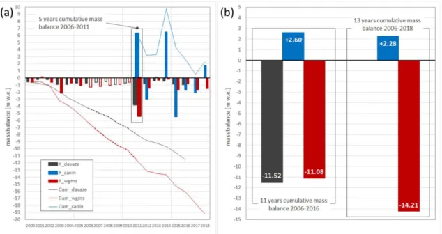
Figure 3. (a) Annual and cumulated geodetic mass balance of the Canin East GIP (Y_canin and Cum_canin) based on a common area (see Figure2for details) compared to 2000–2018 WGMS annual and cumulated mass balance in the Alps (Y_wgms and Cum_wgms) and 2000–2016 optical satellite images annual mass balance calculation based on SLA- METHOD [15] (Y_davaze and cum_davaze) [19]; (b) 11 years (left) and 13 years (right) cumulative mass balance for the three records.

Figure 3. (a) Annual and cumulated geodetic mass balance of the Canin East GIP (Y_canin and Cum_canin) based on a common area (see Figure 2 for details) compared to 2000–2018 WGMS annual and cumulated mass balance in the Alps (Y_wgms and Cum_wgms) and 2000–2016 optical satellite images annual mass balance calculation based on SLA-METHOD [15] (Y_davaze and cum_davaze)[19]; (b) 11 years (left) and 13 years (right) cumulative mass balance for the three records.

It is worth noting that the calculated annual mass balances of the Canin East GIP have a higher uncertainty than the calculated cumulative mass balances. This is because the GIP surfaces for years 2012, 2014 and 2017 were interpolated using GCPs, whereas the calculations of cumulative mass balances are based on LiDAR LiDAR derived DEMs (Ta- bles 1–3). The uncertainty for annual mass balances can be expressed as the maximum positive and negative elevation difference between LiDAR derived DEM through Delau- nay triangulation and GCPs-derived DEM using natural neighbour (Table 3) multiplied by the density of the GIP material, which results in +0.22/−0.28 m w.e.

Figure 4.Surface elevation change of the Canin East GIP for the period 2006–2018 (see colored bar for elevation changes).

Annual surface elevation change recorded between 2011 and 2018 refers to GCP survey, whereas a 5-year and a 12-year surface elevation change reported for the period 2006–2011 and 2006–2018, respectively, refers to Lidar derived surface elevation changes. The GIP outline was adjusted for every surveyed year, and the yearly area change was fully taken into account in the volume change calculations. The large topographic differences observed in some of the surveys, as in the case of the 2012–13, 2013–14 and 2014–15 hydrological years, are due to several different processes able to locally amplify the effect of extreme snow accumulation or ablation: (i) wind snow-blowing; (ii) irregular karst topography due to the presence of karstic shaft, hollows, dolines and canions; (iii) effect of avalanches; (iv) presence of bergschrund.

(11)

Atmosphere2021,12, 263 11 of 25

Figure 4. Surface elevation change of the Canin East GIP for the period 2006-2018 (see colored bar for elevation changes). Annual surface elevation change recorded between 2011 and 2018 refers to GCP survey, whereas a 5-year and a 12-year surface elevation change reported for the period 2006- 2011 and 2006-2018, respectively, refers to Lidar derived surface elevation changes. The GIP outline was adjusted for every surveyed year, and the yearly area change was fully taken into account in the volume change calculations. The large topographic differences observed in some of the surveys, as in the case of the 2012-13, 2013-14 and 2014-15 hydrological years, are due to several different processes able to locally amplify the effect of extreme snow accumulation or ablation: (i) wind snow-blowing; (ii) irregular karst topography due to the presence of karstic shaft, hollows, dolines and canions; (iii) effect of avalanches; (iv) presence of bergschrund.

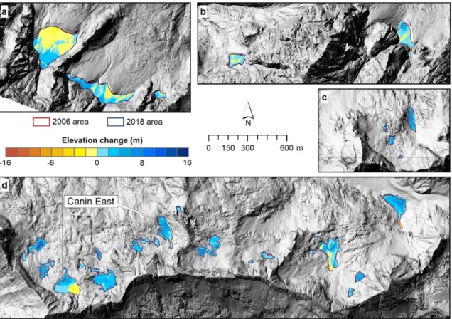
Figure 5. A 12-year (2006–2018) surface elevation change of all the ice bodies in the Italian Julian Alps (see colored bar for elevation changes). (a) Montasio sector. (b) Carnizza-Riofreddo-Studence sector. (c) Cergnala sector. (d) Canin sector.

The volume change of the Canin East GIP for the period 2006–2018 was +43,198 m³, while Montasio West glacier increased by 11,115 m³. The sum of volume change for all the ice bodies in the study area was equal to +479,541 m³.

I

n Figure 3, we compare the mass balance for the period of 2006-2018 observed at the Canin East GIP with data from 239 glaciers in the European Alps using optical satellite images [19] for the period 2000–2016 and with the world glacier monitoring system (WGMS) dataset (WGSM, 2019) from 569 mass balance values with variable time spans for individual glaciers for the period 2000–2018. The strongly positive 2006–2011 cumulative mass balance of the Canin East GIP (+9.41 m w.e.) is in contrast with the strongly negative mass balance of the two alpine datasets (−3.75 m w.e. [19] and −5.36 m w.e.

(WGMS, 2019)). While annual mass balances in 2012, 2013 and 2016 are comparable among the three datasets, they are strongly opposite in 2014 and 2018. In 2015 the Canin East GIP mass balance is about three times more negative than the average in the Alps (Figure 5a). Overall, both the 11-year (2006–2016) and the 13-year (2006–2018) mass balances of the two datasets covering the Alps are strongly negative, whereas during these Figure 5.A 12-year (2006–2018) surface elevation change of all the ice bodies in the Italian Julian Alps (see colored bar for elevation changes). (a) Montasio sector. (b) Carnizza-Riofreddo-Studence sector. (c) Cergnala sector. (d) Canin sector.

It is worth noting that the calculated annual mass balances of the Canin East GIP have a higher uncertainty than the calculated cumulative mass balances. This is because the GIP surfaces for years 2012, 2014 and 2017 were interpolated using GCPs, whereas the calculations of cumulative mass balances are based on LiDAR LiDAR derived DEMs (Tables1–3). The uncertainty for annual mass balances can be expressed as the maximum positive and negative elevation difference between LiDAR derived DEM through Delaunay triangulation and GCPs-derived DEM using natural neighbour (Table3) multiplied by the density of the GIP material, which results in +0.22/−0.28 m w.e.

The volume change of the Canin East GIP for the period 2006–2018 was +43,198 m³, while Montasio West glacier increased by 11,115 m³. The sum of volume change for all the ice bodies in the study area was equal to +479,541 m³.

In Figure 3, we compare the mass balance for the period of 2006–2018 observed at the Canin East GIP with data from 239 glaciers in the European Alps using optical satellite images [19] for the period 2000–2016 and with the world glacier monitoring system (WGMS) dataset (WGSM, 2019) from 569 mass balance values with variable time spans for individual glaciers for the period 2000–2018. The strongly positive 2006–2011 cumulative mass balance of the Canin East GIP (+9.41 m w.e.) is in contrast with the strongly negative mass balance of the two alpine datasets (−3.75 m w.e. [19] and−5.36 m w.e. (WGMS, 2019)). While annual mass balances in 2012, 2013 and 2016 are comparable among the three datasets, they are strongly opposite in 2014 and 2018. In 2015 the Canin East GIP mass balance is about three times more negative than the average in the Alps (Figure5a).

Overall, both the 11-year (2006–2016) and the 13-year (2006–2018) mass balances of the two datasets covering the Alps are strongly negative, whereas during these two periods the mass balance of the Canin Eats GIP and 33 ice bodies of the Italian Julian Alps experienced positive mass balance (Figure5b).

In 2012, when glacier ice outcropped at the end of the ablation season, a set of 7 ablation stakes where drilled by using a Heuke driller in the ice patch (Figure2). Positive mass

(12)

Atmosphere2021,12, 263 12 of 25

balance in 2013 and 2014 kept ablation stakes covered by snow andfirn also during summers 2015, 2016 and until August 2017 when glacier ice outcropped again, and it was therefore possible to measure their topographical position. Only 5 ablation stakes were found, and results show low displacements over the surface of the ice patch with local displacement in the order of 11 to 47 cm in 5 years (i.e., 2 to 10 cm yr⁻¹).

4.3. Winter Meteorological Patterns in Dry and Wet Winters

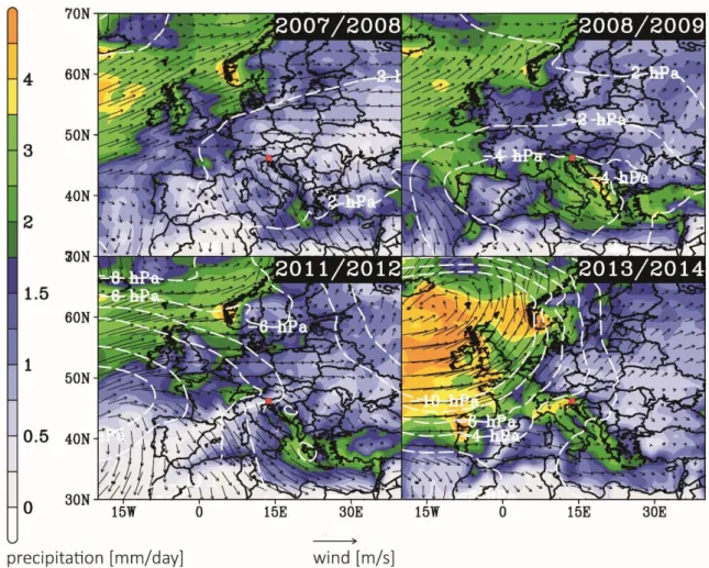
During dry winters, the synoptic conditions generally show relatively high sea level pressure (SLP) anomaly, which in fact can be considered as a high-pressure blocking system (or “blocking high”). This is apparent in the cases of 2007–2008 and 2011–12 (Figure6).

The positive SLP anomaly (reference period: January 1981–January 2010), stable conditions and the downwelling motions together over the southeastern Alps favor the relatively low winter seasonal precipitation.

Figure 6. Mean weather patterns observed over Europe during dry (2006–2007, 2011–2012) and extremely snowy winters (2008–2009, 2013–14). Mean seasonal precipitation (mm/day, colours) and near-surface (10 m) mean seasonal winds (m/s) are represented along with the mean sea level pressure anomalies (reference period: January 1981–January 2010, unit:

hPa). Well-structured and persistent negative sea level pressure anomalies in the Atlantic influenced the regional circulation in Europe and the Mediterranean causing recursive orographic precipitation in the southern Alps, while positive sea level pressure anomalies manifested in low winter precipitation totals. The red square depicts the region of interest.

4.4. Climate Data from Local Observations

Analysis of 1979–2018 climatological records (Figure 7) reveals increasing summer (JJA) temperature over the entire period with no signs of a reversal in the trend. Although the interannual variability is unchanged, both annual minima and maxima show a trend towards warmer values. Summer 2003 (11.3 °C) is the warmest observed, followed by summers 2015, 2012 and 2017, which, all together, are the four hottest summers observed since 1851 [28]. The coolest summer of the last 40 years was 1984 at 6.6 °C. Accordingly, the length and magnitude of the ablation period calculated from the PDD model increased. The number of PDD rose from 169 to 187. The potential melting calculated using a degree day factor for melting snow of 4.0 mm day⁻¹k⁻¹ [60] on average increased about 29 mma⁻¹; from roughly 4119 mm w.e. in the late 1970s to 5279 mm w.e. in the late 2010s.

The less effective ablation seasons were summer 1984 and 1996 with 3446 and 3621 mm w.e., respectively. The most effective ablation seasons, although for different reasons, were in 2003 and 2012 with 5747 and 5755 mm w.e., respectively. Summer 2003 saw the highest recorded temperature for a shorter period, while the 2012 ablation period was longer but less extreme in terms of absolute values. Winter precipitation (wP; DJF) and extended winter precipitation (WP; DJFM) both decreased from late 1970s to the middle 1990s and then increased in the following years. Accordingly, snow total accumulation Figure 6.Mean weather patterns observed over Europe during dry (2006–2007, 2011–2012) and extremely snowy winters (2008–2009, 2013–14). Mean seasonal precipitation (mm/day, colours) and near-surface (10 m) mean seasonal winds (m/s) are represented along with the mean sea level pressure anomalies (reference period: January 1981–January 2010, unit: hPa).

Well-structured and persistent negative sea level pressure anomalies in the Atlantic influenced the regional circulation in Europe and the Mediterranean causing recursive orographic precipitation in the southern Alps, while positive sea level pressure anomalies manifested in low winter precipitation totals. The red square depicts the region of interest.

At the same time, 2008–2009 and 2013–2014 serve as representative examples when during winter extremely abundant precipitation occurred over the southeastern Alps (Figure6). The combination of negative SLP anomaly along with the moist air circulating from the Mediterranean and Adriatic Seas lead to abundant precipitation.

Furthermore, the 2008–2009 winter was characterized by secondary lows forming in the Mediterranean basin with the Alps at the convergence zone of cooler air masses

(13)

Atmosphere2021,12, 263 13 of 25

from North and warmer and moist air masses from the Adriatic and the Mediterranean.

The combination of the aforementioned conditions created one of the snowiest winters in the Eastern Alps since 1930 [62]. On the contrary, in 2013–2014 winter the subpolar low showed a persistent location of its center slightly south east of Iceland inducing advection of mild and wet south-westerly winds over Europe and the Alps. The long-lasting low- pressure region and a secondary cyclogenesis over the Mediterranean caused record- breaking winter snow accumulation in the Eastern Alps [63,64]. More specifically, 2% of the winter Vb cyclones exceed the 95th precipitation percentile in the Alpine region [37], which can lead to abundant winter precipitation as occurred in 2013–2014.

4.4. Climate Data from Local Observations

Analysis of 1979–2018 climatological records (Figure7) reveals increasing summer (JJA) temperature over the entire period with no signs of a reversal in the trend. Although the interannual variability is unchanged, both annual minima and maxima show a trend towards warmer values. Summer 2003 (11.3^◦C) is the warmest observed, followed by summers 2015, 2012 and 2017, which, all together, are the four hottest summers observed since 1851 [28]. The coolest summer of the last 40 years was 1984 at 6.6^◦C. Accordingly, the length and magnitude of the ablation period calculated from the PDD model increased.

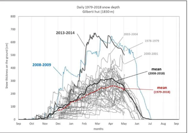
The number of PDD rose from 169 to 187. The potential melting calculated using a degree day factor for melting snow of 4.0 mm day⁻¹k⁻¹[60] on average increased about 29 mma⁻¹; from roughly 4119 mm w.e. in the late 1970s to 5279 mm w.e. in the late 2010s. The less effective ablation seasons were summer 1984 and 1996 with 3446 and 3621 mm w.e., respectively. The most effective ablation seasons, although for different reasons, were in 2003 and 2012 with 5747 and 5755 mm w.e., respectively. Summer 2003 saw the highest recorded temperature for a shorter period, while the 2012 ablation period was longer but less extreme in terms of absolute values. Winter precipitation (wP; DJF) and extended winter precipitation (WP; DJFM) both decreased from late 1970s to the middle 1990s and then increased in the following years. Accordingly, snow total accumulation (STA) shows a similar behavior. The two highest STAs recorded since 1972 were the winters of 2013–2014 (15.67 m) and 2008–2009 (13.52 m). Hence, although both summer temperature and ablation period became gradually less favorable for snow and ice preservation, the envELA stabilized in the 2000s highlighting a decreasing trend between 2003 and 2011 when it reached values as low as in the late 1980s. The 2014 envELA at 1917 m was the lowest of the last 40 years, while the 2003 envELA at 3262 m was the highest. Analysis of the 1979–2018 daily snow depth measured at Gilberti weather station (Figure8) reveals that the winters 2008–2009 and 2013–2014 both represent extreme events in the recent snow-climatology of this area with roughly double the long-term mean snow depth. Such values, measured at 1830 m a.s.l., are to be considered as an underestimation of the real snow amount fallen over the accumulation area of most of the ice patches and glaciers located at higher altitude and where most favorable topo-climatic conditions led to increase snow-accumulation.

The winters 2000–2001 and 2003–2004 also recorded much-higher-then-average snow accumulation, as well as winter 1979–1980.

(14)

Atmosphere2021,12, 263 14 of 25

(STA) shows a similar behavior. The two highest STAs recorded since 1972 were the winters of 2013–2014 (15.67 m) and 2008–2009 (13.52 m). Hence, although both summer temperature and ablation period became gradually less favorable for snow and ice preservation, the envELA stabilized in the 2000s highlighting a decreasing trend between 2003 and 2011 when it reached values as low as in the late 1980s. The 2014 envELA at 1917 m was the lowest of the last 40 years, while the 2003 envELA at 3262 m was the highest. Analysis of the 1979–2018 daily snow depth measured at Gilberti weather station (Figure 8) reveals that the winters 2008–2009 and 2013–2014 both represent extreme events in the recent snow-climatology of this area with roughly double the long-term mean snow depth. Such values, measured at 1830 m a.s.l., are to be considered as an underestimation of the real snow amount fallen over the accumulation area of most of the ice patches and glaciers located at higher altitude and where most favorable topo-climatic conditions led to increase snow-accumulation. The winters 2000–2001 and 2003–2004 also recorded much- higher-then-average snow accumulation, as well as winter 1979–1980.

Figure 7. Climatic data observed in the 40 years period 1979–2018: (a) summer air temperature (JJA); (b) winter precipitation (djf; wP) and extended winter precipitation (djfm; WP) and snow total accumulation (STA); (c) environmental ELA [15,17]; (d) number of positive degree days and PDD sum.

Figure 7.Climatic data observed in the 40 years period 1979–2018: (a) summer air temperature (JJA); (b) winter precipitation (djf; wP) and extended winter precipitation (djfm; WP) and snow total accumulation (STA); (c) environmental ELA [15,17];

(d) number of positive degree days and PDD sum.

(15)

Atmosphere2021,12, 263 15 of 25

Figure 8. Daily snow thickness recorded at the Gilberti weather station (1830 m asl). The light grey lines show individual years, with the exceptional years of 1978–1979, 2000–2001 and 2003–2004 indicated. Black-bold curve is the 2008–2018 mean, while the red-dotted line is the 1979–2008 mean (limited to the period 1 Dec–30 April). The latter represents the longest snow record of the Gilberti weather station. Note how the 2008-2018 mean lies above the longer-term mean for 1979–2018.

5. Discussion

Although the variability of winter precipitation and glacier accumulation is strongly related to the NAO in Scandinavia and Svalbard, with the AMO also influencing the northernmost glaciers [65,66], this signal over the Alps is somewhat contradictory. Mar- zeion and Nesje (2012) [67] showed that the NAO in the western Alps is weakly anti-correlated with the mass balance of glaciers due to temperature and winter precipitation anomalies. In the Julian Alps, located in the south-east side of the alpine chain, there is no evidence of correlation between NAO and the past and recent evolution of ice bodies (r^s= 0.09; Figure S2). Looking at the long-term evolution of alpine glaciers, Huss et al. (2010) [43]

found that glacier mass budget in the Swiss Alps varied in phase with the AMO and is therefore strictly related to North Atlantic variability, but associated with the ongoing global warming. Their results also suggest how the size of glaciers in the Alps reacted in response to AMO-driven variations at least over the last 250 years. They also stated that at the regional alpine scale, AMO is thought to influence the mass budget of glaciers mainly through minima and maxima in temperature of the ablation season.

Regular position measurements of the Canin East glacier terminus from fixed bench- marks started in 1896 [68] and continued through the 20th century up to the present days, with only occasional interruptions during the 1st and 2ndWorld War [28]. Comparison of glacier-length variation with the AMO index and the normalized MSAT recorded at 2200 m a.s.l. in the Julian Alps over the time window 1851–2018 (Figure 9) show how multidecadal variations are in phase with AMO with a very strong statistically significance correlation (Sperman’s test; rs = −0.94; p < 0.05), whereas the statistic significance with the extended-winter (djfm) 1920–2018 precipitation is weaker (rs = 0.29; p < 0.005). Advances and Figure 8.Daily snow thickness recorded at the Gilberti weather station (1830 m asl). The light grey lines show individual years, with the exceptional years of 1978–1979, 2000–2001 and 2003–2004 indicated. Black-bold curve is the 2008–2018 mean, while the red-dotted line is the 1979–2008 mean (limited to the period 1 December–30 April). The latter represents the longest snow record of the Gilberti weather station. Note how the 2008–2018 mean lies above the longer-term mean for 1979–2018.

5. Discussion

Although the variability of winter precipitation and glacier accumulation is strongly related to the NAO in Scandinavia and Svalbard, with the AMO also influencing the northernmost glaciers [65,66], this signal over the Alps is somewhat contradictory. Marzeion and Nesje (2012) [67] showed that the NAO in the western Alps is weakly anti-correlated with the mass balance of glaciers due to temperature and winter precipitation anomalies.

In the Julian Alps, located in the south-east side of the alpine chain, there is no evidence of correlation between NAO and the past and recent evolution of ice bodies (rs= 0.09;

Figure S2). Looking at the long-term evolution of alpine glaciers, Huss et al. (2010) [43]

found that glacier mass budget in the Swiss Alps varied in phase with the AMO and is therefore strictly related to North Atlantic variability, but associated with the ongoing global warming. Their results also suggest how the size of glaciers in the Alps reacted in response to AMO-driven variations at least over the last 250 years. They also stated that at the regional alpine scale, AMO is thought to influence the mass budget of glaciers mainly through minima and maxima in temperature of the ablation season.

Regular position measurements of the Canin East glacier terminus from fixed bench- marks started in 1896 [68] and continued through the 20th century up to the present days, with only occasional interruptions during the 1st and 2nd World War [28]. Comparison of glacier-length variation with the AMO index and the normalized MSAT recorded at 2200 m a.s.l. in the Julian Alps over the time window 1851–2018 (Figure9) show how multidecadal variations are in phase with AMO with a very strong statistically significance correlation (Sperman’s test; rs=−0.94;p< 0.05), whereas the statistic significance with the extended-

(16)

Atmosphere2021,12, 263 16 of 25

winter (djfm) 1920–2018 precipitation is weaker (rs= 0.29;p< 0.005). Advances and retreats of the Canin East glacier terminus are in phase with the AMO (Figure9), which explains almost 120 years of glacier oscillation in the Julian Alps very well. Short periods of glacier advances recorded in 1910–1920 and 1945–1975, as well as in the 1930s, are very well linked and modulated by drops in MSAT. Spearman’s correlation test between the two variables returns a moderate to strong correlation (rs=−0.63p< 0.05). The fast and steady increase in MSAT from early 1980s due to anthropogenic global warming is superimposed to the AMO and explains the dramatic glacier reduction that is particularly evident after the 1980s.

retreats of the Canin East glacier terminus are in phase with the AMO (Figure 9), which explains almost 120 years of glacier oscillation in the Julian Alps very well. Short periods of glacier advances recorded in 1910–1920 and 1945–1975, as well as in the 1930s, are very well linked and modulated by drops in MSAT. Spearman’s correlation test between the two variables returns a moderate to strong correlation (r^s= −0.63 p < 0.05). The fast and steady increase in MSAT from early 1980s due to anthropogenic global warming is superimposed to the AMO and explains the dramatic glacier reduction that is particularly evident after the 1980s.

Figure 9. (a) Winter (DJFM) precipitation [28]; (b) summer (JJA) temperature [28]; (c) AMO index and observed length change of Canin East glacier (https://www.esrl.noaa.gov/psd/data/timeseries/AMO;

Last accessed August 2020). Bold lines indicate a 11-year low-pass filter, Red line in (c) refers to glacier length while blue line to AMO index.

The almost perfect match of glacier reaction to summer temperature forcing, without any apparent delay as in the case of larger alpine valley glaciers, is likely due to the small size of the ice body, which led to a short reaction time (<2 yr) in response to climatic variability [69]. Although both AMO and MSAT explain well the long-term glacier variability in the Julian Alps in agreement with what has been observed in the Alps so far, the recent Figure 9.(a) Winter (DJFM) precipitation [28]; (b) summer (JJA) temperature [28]; (c) AMO index and observed length change of Canin East glacier (https://www.esrl.noaa.gov/psd/data/timeseries/

AMO; Last accessed 5 August 2020). Bold lines indicate a 11-year low-pass filter, Red line in (c) refers to glacier length while blue line to AMO index.

The almost perfect match of glacier reaction to summer temperature forcing, without any apparent delay as in the case of larger alpine valley glaciers, is likely due to the small size of the ice body, which led to a short reaction time (<2 yr) in response to climatic variability [69]. Although both AMO and MSAT explain well the long-term glacier variability in the Julian Alps in agreement with what has been observed in the Alps so far,

(17)

Atmosphere2021,12, 263 17 of 25

the recent drop in envELA and the positive mass balance 2006–2018 are in contrast with what is globally reported elsewhere in the Alps [12].

The general increase in winter (DJFM) precipitation after the negative anomaly of the 1990s (Figure9a) and the 2008–2009 and 2013–2014 extremes (Figure8), which brought much higher than average snow accumulation over the ice bodies, are responsible for the observed ice bodies stability and for the 2006–2018 positive mass balance. Recent positive mass balance cannot be attributed to favorable temperature because summers have become longer and hotter (Figure7d) increasing the snow/ice melting on average by about 29 mm a⁻¹since 1979 according to the DDM (Figure7d). Spearman’s correlation analysis between the observed 2006–2018 mass balance and the PDD model results shows a moderate correlation statistically not significant (rs=−0.45;p= 0.26). The observed lowering of the envELA in the 2000s, which brought ice body stability and recovery, is therefore due only to changes in precipitation regime and, particularly, in the occurrence of few extreme winter accumulation seasons. This circumstance influenced the fate of ice bodies in the Julian Alps for several years also thanks to the short (<2 yr) metamorphosis of snow into ice. This finding is consistent with Spearman’s correlation test between the 2006–2018 annual mass balance and the winter (djfm) precipitation as well as winter (djfma) snowfall, giving a very strong correlation statistically significant (rs= 0.91;p< 0.005 and rs= 0.74;

p< 0.05, respectively). Extreme winter accumulation seasons led to multi-annual snow metamorphism and formation of new ice as reported at the end of very hot summers which led to highly negative mass balance in 2012 and 2016. In those years when all previous winter snow was totally removed by melting, bare ice outcropped over the entire surface of the ice patch. The topographic position of ablation stakes indicates a weak dynamics of the Canin East GIP, which is typical of mass movement of ice patches [1] rather than glacier movement due to internal deformation and flow as reported from Montasio glacier by [2,30].

Montasio glacier is the only one to present well defined accumulation and ablation areas (Figure4), whereas the other ice patches of the Julian Alps do not present a clear ELA.

The reason is ascribable to the local topography and the present size of the ice bodies.

Snow accumulation due to avalanches affects only the upper part of Montasio glacier, while other Julian Alps ice bodies are often affected by avalanche activity along their entire surface. The dominant role played by solid precipitation in regulating the recent annual mass balance of Montasio glacier as well as the statistically non-significant correlation with temperature of the ablation season was recently also reported by De Marco et al. 2020 [30].

Observations from glaciers in the Austrian Alps (Abermann, Kuhn and Fischer, 2011) confirmed this finding further, suggesting that a slowdown in glacier recession in this area might be related to “above average accumulation”. By dividing the Alps into different sub- regions, each one identified from 2000–2016 annual mass balance time series, Davaze et al.

(2020) [15] found that the only climatic parameter statistically significant explaining more than 30% of the observed inter-annual mass balance variance in the Central and Eastern Alps and Tyrol is the precipitable water during winter, that combined with temperature, influences winter precipitation amount.

It has previously been reported how the maritime glaciers in the Julian Alps recently showed higher climatic sensitivity to precipitation than to air temperature (Colucci and Guglielmin, 2015) (Salvatore et al., 2015). Other authors recently highlighted how residual ice masses in other maritime areas (i.e., where MAP is high) in the southern Alps showed contradictory signs of stability and/or shrinking slow down instead of rapidly disappearing as might be expected (Scotti and Brardinoni, 2018).

Topoclimatic factors and the role of wind-blown and avalanche-fed accumulation (Fischer, 2011) (Luca Carturan et al., 2013) (Colucci, 2016) (Colucci and Žebre, 2016) (Hughes, 2018) (Baroni, Carlo, Bondesan, Aldino, Carturan, Luca, Chiarle, 2019), topographic influence and the geometry of the ice body (Colucci, 2016) (Scotti and Brardinoni, 2018) (De Marco et al., 2020) as well as higher sensitivity of precipitation in areas where MAP are the highest (Colucci and Guglielmin, 2015) collectively account for such anomaly.