rspb.royalsocietypublishing.org
Research
Cite this article:
Kocsis A´T, Reddin CJ, Kiessling W. 2018 The biogeographical imprint of mass extinctions.
Proc. R. Soc. B 285:20180232.
http://dx.doi.org/10.1098/rspb.2018.0232
Received: 29 January 2018 Accepted: 11 April 2018
Subject Category:
Palaeobiology
Subject Areas:
evolution, ecology, palaeontology
Keywords:
benthic, palaeobiology, mass extinctions, bioregions, networks
Author for correspondence:
A´da´m T. Kocsis
e-mail: adam.kocsis@fau.de
Electronic supplementary material is available online at https://doi.org/10.6084/m9.figshare.
c.4070987.
The biogeographical imprint of mass extinctions
A´da´m T. Kocsis
1,2, Carl J. Reddin
1and Wolfgang Kiessling
11GeoZentrum Nordbayern, Department of Geography and Geosciences, University of Erlangen-Nuremberg, Loewenichstraße 28, 91054 Erlangen, Germany
2MTA-MTM-ELTE Research Group for Paleontology, POB 137, 1431 Budapest, Hungary A´TK, 0000-0002-9028-665X; CJR, 0000-0001-5930-1164; WK, 0000-0002-1088-2014
Mass extinctions are defined by extinction rates significantly above back- ground levels and have had substantial consequences for the evolution of life. Geographically selective extinctions, subsequent originations and species redistributions may have changed global biogeographical structure, but quantification of this change is lacking. In order to assess quantitatively the bio- geographical impact of mass extinctions, we outline time-traceable bioregions for benthic marine species across the Phanerozoic using a compositional net- work. Mass extinction events are visually recognizable in the geographical depiction of bioregions. The end-Permian extinction stands out with a severe reduction of provinciality. Time series of biogeographical turnover represent a novel aspect of the analysis of mass extinctions, confirming concentration of changes in the geographical distribution of benthic marine life.
1. Introduction
Mass extinctions, defined as extinction rates significantly above background, punctuated the history of life on Earth [1]. These cataclysmic events obliterated the majority of species [2], altered ecosystem structures [3] including the replace- ment of incumbent clades [4,5], but were surprisingly reserved in altering functional diversity [6]. The transient loss of biodiversity associated with bottle- neck effects on surviving lineages [7] and survivor redistribution [8] are expected to change the biogeographical structure of the biosphere, but there are limited data supporting this conjecture.
We expect the turnover of global biogeographical structures, from inter- vals preceding mass extinctions to intervals following them, to be significantly higher than for background intervals. This hypothesis stands regardless of the direct extinction mechanism. Species extinctions, combined with the proliferation of ‘disaster taxa’ with wider geographical ranges [9] in low diversity communities [10] should lead to a biogeographically more uniform world. Furthermore, uneven geographical extinction selectivity during mass extinctions [11,12] should be apparent through the survival of bioregions. A decrease in beta diversity is sometimes noted after extinction events [13,14] but not uniformly so ([15], fig. 5).
In order to clarify the biogeographical imprint of mass extinctions, we applied a novel method of assessing biogeographical turnover through geological ages.
Using a biogeographical network approach [12,16–18], we analysed the global spatio-temporal structure of the marine fossil record and outlined time-traceable bio- geographical units (bioregions). We constructed time series of the changes between consecutive geographical renderings (by-cell spatio-temporal turnover) and of the secular emergence and disintegration of the biogeographical units (by-bioregion temporal turnover). We quantitatively confirm that mass extinctions were associated with elevated biogeographical reorganization of marine benthic species.
2. Data and methods (a) Data
Occurrences of marine invertebrate species were downloaded from the Paleobiology Database (PaleoDB, http://paleobiodb.org) on 7 July 2017 and parsed into one of
&
2018 The Author(s) Published by the Royal Society. All rights reserved.Downloaded from https://royalsocietypublishing.org/ on 16 November 2021
82 geological ages (see electronic supplementary material). The downloaded taxa included the well-preserved benthic ‘core’
groups of Brachiopoda, Bivalvia, Gastropoda, Bryozoa, Echinoder- mata, Anthozoa, Decapoda and Trilobita. The dataset comprised 370 459 fossil occurrences of 87 618 species. Palaeo-geographical coordinates were obtained by rotating the present day coordinates of fossil collections with the GPlates 2.0.0 software with the rotation file supplied by C. Scotese in the ‘PALEOMAP PaleoAtlas for GPlates’ package [19]. After the coordinates were calculated, the collections were binned using an icosahedral geographical grid from the ‘icosa’ R package [20] with 362 roughly equal area cells (tessellation level¼6, mean cell area¼1 409 021 km2). To construct a time-uniform biogeographical partitioning scheme, we assigned the fossil occurrences to spatio-temporal units, i.e.
time bin-specific geographical grid where the combination of the geographical cell and time slice variables represent the units used in the network analysis. Out of the 29 684 spatio-temporal cells (82 post-Cambrian ages362 geographical cells) available for occupation, 2117 contained more than 10 occurrences, which was our minimum quota for sampling.
(b) Network analysis
Using the species shared between the 2117 spatio-temporal units, we constructed a bipartite occurrence network [16,21]. After pro- jection to represent only the spatio-temporal units as vertices, the weights of the network edges were adjusted for sampling intensity following Rojaset al. [17]. Using this single network, we outlined partitions with the ‘infomap’ community detection algorithm (see electronic supplementary material, [22]). The resulting mod- ules of the network represented spatially coherent bioregions (biogeographical units) that can be traced through time [23].
(c) Turnover
Three kinds of faunal turnover were considered in the study:
(1) by-cell (total biogeographical turnover); (2) by-bioregion (emer- gence and disintegration) and (3) taxonomic (species origination and extinction). The total temporal heterogeneity of the biogeogra- phical changes, (1), was described using differences between the geographical renderings of bioregions in consecutive time bins.
We defined by-cell biogeographical turnover from time bini21 toias the proportion
bi¼ ndiffi
nsampi , ð2:1Þ
wherensampi represents the number of geographical cells sampled in both time bini21 andi, whereasndiffi denotes the number of cells among these that changed bioregion membership. This approach allowed us to constrain turnover between 0 (no change) and 1 (complete turnover). An advantage of this metric is that although non-random sampling can influence it, the number of sampled cells is not expected to have a predictable effect on the trueness of the estimates.
We also tallied the emergence (‘origination’) and disintegration (‘extinction’) of bioregions and expressed them as proportions to the total number of outlined bioregions in the slice (2, by-bioregion turnover). Single-interval bioregions were excluded to avoid spur- ious correlations between the emergence and disintegration series.
As varying sampling intensity can bias this metric, we calculated these proportions with subsampling to the same number of geographical cells.
To contrast biogeographical patterns with taxonomic turnover, species-level taxonomic extinction and origination rates (3), were calculated both with the rawper capita[24] and the subsampled gap-filler rate equations [25]. The dataset was subsampled with classical rarefaction to overcome biases introduced by the chan- ging sampling intensity (electronic supplementary material). All analyses were carried out in the R environment [26].
3. Bioregion changes at mass extinction intervals
The traditional ‘Big Five’ mass extinction intervals [1] are apparent on the time series of maps displaying the changing fabric of bioregions through time (figure 1). Besides substantial changes of geographical cell memberships, the end-Permian mass extinction figures prominently in a dramatic loss of pro- vinciality. This devastating event led to a world without any observable biogeographical structure of marine macrobenthic animals, and it represents the minimum of the number of out- lined bioregions in the Phanerozoic (electronic supplementary material, table S1).
The disintegration of bioregions was not uniform during mass extinctions and subsequent reorganization featured great geographical variability. This pattern has been suggested for the end-Cretaceous mass extinction [8], which preferen- tially disrupted American marine bioregions, and had less effect on the other side of the Atlantic. The southern polar bio- regions persisted through the end-Triassic and end-Cretaceus events, which conforms to the hypothesis of greater extinction toll in the tropics during these intervals [11,12]. A similarly selective disintegration is evident through the end-Devonian extinctions; only the Laurentian biogeography appears to have been affected by the Frasnian/Famennian event, while cells in the Palaeotethys exhibit more drastic membership changes after the end of the Famennian age. On the other hand, only the first pulse of the end-Ordovician extinction (start of the glaciation) is associated with major biogeographi- cal changes [14]. The biogeographical turnover was elevated at the Katian/Hirnantian transition, coinciding with the spread of theHirnantiafauna [27], and was only mild at the end of the Ordovician period.
The apparently uniform structure in the earliest Triassic is likely related to the expanded distribution of cosmopolitan species that filled up niche-space opened up by the mass extinc- tion. Besides some prominent examples of disaster species (e.g.Claraia clarai[28]), broader ranges are also suggested by the elevated occupancies of the earliest Triassic faunal elements [29]. However, as similarly high occupancies were suggested for the Late Permian [29], the pronounced provinciality of this interval (figure 1c) may indicate that changes in the overlap patterns of geographical ranges contributed to the loss of bio- geographical structure. As disaster species are opportunistic by definition [10], they can create gradually overlapping distri- butions over a wider variety of environments, resembling randomly placed species in a continuous habitat space. The pattern of increasing extinction-related cosmopolitanism is also observable in the terrestrial environment [9], which was likely followed by an increase in provincialisation, as in the record of tetrapods [18]. The development of a latitudinal gra- dient in ammonoid diversity in the Early Triassic [30] is also an example of this biogeographical rebound process.
4. Biogeographical turnover through time
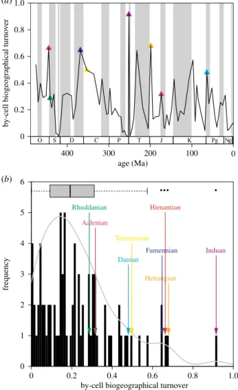
In order to relate the magnitude of biogeographical changes at mass extinctions to those of background-intervals, we traced biogeographical turnover through the Phanerozoic. Although there is no significant trend of by-cell biogeographical turnover through time (figure 2a, Spearman rank-order correlation with timer¼0.15,p¼0.1811,n¼81), by-cell turnover is sig- nificantly correlated with the corresponding species-level
rspb.r oy alsocietypublishing.org Pr oc. R. Soc. B 285 : 20180232
2
Downloaded from https://royalsocietypublishing.org/ on 16 November 2021
extinction rates (r¼0.52,p,0.0001, electronic supplementary material). The distribution of by-cell biogeographical turnover is slightly right skewed (figure 2b), similar to that of taxonomic turnover rates [31].
Changes in the biogeographical structure of the benthic environment are concentrated at mass extinction boundaries (figure 2b). The intervals following the ‘Big Five’ (figure 2) are characterized by significantly higher biogeographical turn- over (Wilcoxon rank sum testW¼493, p,0.0001) than the rest of the intervals. The background turnover process changed the biogeographical membership of about 17% of the benthic habitat area per geological age. During mass extinction inter- vals the median turnover value rose to 63%. The aftermath of the Early Jurassic Anoxic Event [32] is also associated with elevated biogeographical turnover, along with some other
intervals (Carnian and Cenomanian), which are not known to coincide with severe extinction episodes. Subsampling simu- lations (electronic supplementary material) suggest that these peaks are not introduced by changes of species richness.
The by-cell biogeographical turnover reflects the combined effect of bioregion relocations, disintegration of bioregions in the extinction interval, and emergence of new bioregions in the aftermath. Both the emergences and disintegrations of bio- regions (figure 3) are associated with elevations of species extinction and origination rates, but the emergences contribute more to the by-cell turnover signal over all ages (electronic sup- plementary material text). During the crisis intervals related to the ‘Big Five’, however, disintegration and emergence values were on par in driving the total changes in biogeography (paired Wilcoxon rank-sum test between emergence and
17 17
17
29
19
19
N/A N/A
N/A 17 1717
17 N/A
19
17 N/A
17 N/A
17 17
1919
19
N/A 17
19
29 N/A
19 19
19 29
19 19
19 29
N/A
N/A
N/A
N/A N/A
N/A 17
1717 17
17
19 N/A
19 19
19 19
19 19
N/A 19
N/A
N/A
7575
N/A 29
19
19 N/A N/A
19
19
N/A 19
N/A N/A
N/A 19
7
7
19 19
7 N/A
19 19
N/A 19
N/A
19 19
19 19
N/A
51 51
7 20
20
20 6 6
2020 20 N/A
20
6
20 6
N/A 6
6 N/A
20
6 6 51
51
20 N/A 6
N/A 6
6 6
20 N/A N/A
N/A
6 6 N/A N/A
6
N/A
6 6 6
6
N/A
N/A 2024 6
20 84
6 2424
24 24
N/A 6
N/A
6 21 9
N/A 6 N/A
6
6
6 6
N/A N/A N/A
N/A
24
46 21
24 24
24 21
24
N/A
N/A
21
46 21
N/A
46 N/A
N/A 24
N/A
N/A
N/A21 N/A
24 21N/A
N/A
N/A N/A
N/A 21
1 1
1 1 1
15
15 1
1
1
1 N/A 1
1 1
N/A 1
1
1
1 N/A
N/A 1 N/A
1 N/A 36
1
N/A
N/A N/A
N/A 36 N/A
1 1 N/A
9
N/A
N/A N/A
N/A
N/A 1
N/A N/A
N/A 1
1
15 15
1 1 1
N/A 1
N/A
1 N/A 11
1
9
1
1
1
N/A 1
1 N/A
36
1
N/A N/A
N/A N/A
N/A N/A
N/A 36
N/A N/A
N/A N/A
N/A 11 11
11 N/A 11
11
11 11
11 11
N/A
N/A 11
N/A 11 11
N/A 11
11 N/A
N/A 11
N/A N/A
N/A
11
11 N/A
N/A
N/A N/A N/A
13
13 13
13 N/A
28
28 13
13
13 13
13
13
N/A
N/A 1313
N/A 11
13
28 N/A
N/A N/A
N/A
13 N/A
28 N/A N/A
13
13 13
13 13 N/A
13
13 13
13
13 13
13 13
13 13
13 N/A
N/A N/A
N/A N/A
N/A 13 N/A
N/A
N/A N/A
N/A N/A
13 1313
13 13
13
N/A
13 N/A
2 N/A 13
N/A
28 28
2
N/A
13 13 N/A
N/A 13
N/A
28 13 N/A
13
N/A N/A
64 64 N/A 64
N/A
28 13
N/A
N/A 13
31 18
18 3
18 18
31
3 3
18
3 N/A 31
18
18 3
62
32 N/A
3
N/A
32 3
N/A 3 N/A
N/A N/A
N/A N/A
N/A N/A
N/A
27 27
3 N/A
N/A
3 3
N/A 3
3 3
N/A 3
N/A 3
N/A
27 3
3 3
3
3 3
3
27
3
3
27
N/A
32
3 3
3
3 27
N/A 3 3
3 3
3 3
3
3 3 3 3 3
3
3 3
N/A
3 N/A
3 N/A N/A
N/A N/A
N/A N/A N/A
N/A
N/A 18 18
181818
18
32
32 18
62
32 31
32 N/A
32 31
3 3
62 31 18
62 N/A
N/A N/A
N/A
14
3 3 3
3
32 32 14
N/A N/A
14 3 34
14
N/A 3
N/A
32 32
18
3
14
10 3
3 N/A 3
3 N/A N/A N/A
N/A N/A
16
N/A N/A
N/A
2
2 2 2 2 N/A N/A
N/A 2
63 N/A
28 2
N/A
2
N/A
2 2
N/A N/A
2
end-Ordovician ME ME
ME ME
ME
ME
ME
Ordovician, Katian stage (451 Ma) Ordovician, Hirnantian stage (445 Ma) Silurian, Rhuddanian stage (441 Ma)
Permian, Wuchiapingian stage (257 Ma)
Triassic, Norian stage (218 Ma)
Cretaceous, Campanian stage (77 Ma) Cretaceous, Maastrichtian stage (68 Ma) Palaeogene, Danian stage (64 Ma)Palaeogene, Danian stage (64 Ma) end-Cretaceous
end-Devonian
end-Permian
end-Triassic
Triassic, Rhaetian stage (205 Ma) Jurassic, Hettangian stage (199 Ma) Devonian, Frasnian stage (380 Ma) Devonian, Famennian stage (368 Ma)
Permian, Changshingian stage (253 Ma) Triassic, Induan stage (251 Ma) Carboniferous, Tournaisian stage (353 Ma)
(e) (b) (a)
(c)
(d)
17 17
17
29
19
19
N/A N/A
N/A 17 1717
17 N/A
19
17 N/A
17 N/A
17 17
1919
19
N/A 17
19
29 N/A
19 19
19 29
19 19
19 29
N/A
N/A
N/A
N/A N/A
N/A 17
1717 17
17
19 N/A
19 19
19 19
19 19
N/A 19
N/A
N/A
7575
N/A 29
19
19 N/A N/A
19
19
N/A 19
N/A N/A
N/A 19
7
7
19 19
7 N/A
19 19
N/A 19
N/A
19 19
19 19
N/A
51 51
7 20
20
20 6 6
2020 20 N/A
20
6
20 6
N/A 6
6 N/A
20
6 6 51
51
20 N/A 6
N/A 6
6 6
20 N/A N/A
N/A
6 6 N/A N/A
6
N/A
6 6 6
6
N/A
N/A 2024 6
20 84
6 2424
24 24
N/A 6
N/A
6 21 9
N/A 6 N/A
6
6
6 6
N/A N/A N/A
N/A
24
46 21
24 24
24 21
24
N/A
N/A
21
46 21
N/A
46 N/A
N/A 24
N/A
N/A
N/A21 N/A
24 21N/A
N/A
N/A N/A
N/A 21
1 1
1 1 1
15
15 1
1
1
1 N/A 1
1 1
N/A 1
1
1
1 N/A
N/A 1 N/A
1 N/A 36
1
N/A
N/A N/A
N/A 36 N/A
1 1 N/A
9
N/A
N/A N/A
N/A
N/A 1
N/A N/A
N/A 1
1
15 15
1 1 1
N/A 1
N/A
1 N/A 11
1
9
1
1
1
N/A 1
1 N/A
36
1
N/A N/A
N/A N/A
N/A N/A
N/A 36
N/A N/A
N/A N/A
N/A 11 11
11 N/A 11
11
11 11
11 11
N/A
N/A 11
N/A 11 11
N/A 11
11 N/A
N/A 11
N/A N/A
N/A
11
11 N/A
N/A
N/A N/A N/A
13
13 13
13 N/A
28
28 13
13
13 13
13
13
N/A
N/A 1313
N/A 11
13
28 N/A
N/A N/A
N/A
13 N/A
28 N/A N/A
13
13 13
13 13 N/A
13
13 13
13
13 13
13 13
13 13
13 N/A
N/A N/A
N/A N/A
N/A 13 N/A
N/A
N/A N/A
N/A N/A
13 1313
13 13
13
N/A
13 N/A
2 N/A 13
N/A
28 28
2
N/A
13 13 N/A
N/A 13
N/A
28 13 N/A
13
N/A N/A
64 64 N/A 64
N/A
28 13
N/A
N/A 13
31 18
18 3
18 18
31
3 3
18
3 N/A 31
18
18 3
62
32 N/A
3
N/A
32 3
N/A 3 N/A
N/A N/A
N/A N/A
N/A N/A
N/A
27 27
3 N/A
N/A
3 3
N/A 3
3 3
N/A 3
N/A 3
N/A
27 3
3 3
3
3 3
3
27
3
3
27
N/A
32
3 3
3
3 27
N/A 3 3
3 3
3 3
3
3 3 3 3 3
3
3 3
N/A
3 N/A
3 N/A N/A
N/A N/A
N/A N/A N/A
N/A
N/A 18 18
181818
18
32
32 18
62
32 31
32 N/A
32 31
3 3
62 31 18
62 N/A
N/A N/A
N/A
14
3 3 3
3
32 32 14
N/A N/A
14 3 34
14
N/A 3
N/A
32 32
18
3
14
10 3
3 N/A 3
3 N/A N/A N/A
N/A N/A
16
N/A N/A
N/A
2
2 2 2 2 N/A N/A
N/A 2
63 N/A
28 2
N/A
2
N/A
2 2
N/A N/A
2
end-Ordovician ME ME
ME ME
ME
ME
ME
Ordovician, Katian stage (451 Ma) Ordovician, Hirnantian stage (445 Ma) Silurian, Rhuddanian stage (441 Ma)
Permian, Wuchiapingian stage (257 Ma)
Triassic, Norian stage (218 Ma)
Cretaceous, Campanian stage (77 Ma) Cretaceous, Maastrichtian stage (68 Ma) end-Cretaceous
end-Devonian
end-Permian
end-Triassic
Triassic, Rhaetian stage (205 Ma) Jurassic, Hettangian stage (199 Ma) Devonian, Frasnian stage (380 Ma) Devonian, Famennian stage (368 Ma)
Permian, Changshingian stage (253 Ma) Triassic, Induan stage (251 Ma) Carboniferous, Tournaisian stage (353 Ma)
(e) (b) (a)
(c)
(d)
Figure 1.
Geographical positions of bioregions before and after the traditional ‘Big Five’ mass extinctions [1]. Dashed vertical lines indicate mass extinction bound- aries. The end-Ordovician and end-Devonian extinctions comprise three stages. Numbers and colours indicate time-traceable bioregions. N/A entries denote cells with inadequate sampling (less than 10 occurrences). Maps are the PALEOMAP raster series of C. Scotese [19].
rspb.r oy alsocietypublishing.org Pr oc. R. Soc. B 285 : 20180232
3
Downloaded from https://royalsocietypublishing.org/ on 16 November 2021
disintegration values related to the extinction pulses shown in
figure 1,
W¼28, p¼0.7209). The end-Ordovician, end-Permian, end- Triassic and end-Cretaceous mass extinctions are characterized by elevated bioregion disintegration values (figure 3).
Large-scale shifts of sampling and the sometimes poor spatial coverage of fossil occurrences challenge the evaluation of provinciality. However, higher-level descriptors, such as biogeographical turnover are stable across multiple spatial resolutions (electronic supplementary material, figures S1 and S2), incorporating the lower-level result instability as randomly distributed error.
Changes in biogeography can be assessed in a similar fashion to taxonomic turnover, and species extinctions are sig- nificantly cross-correlated with biogeographical turnover. As we outlined bioregions using species composition data, the tra- jectory of biogeographical turnover inherently carries a signal of species turnover. Although temporal clusters of the fauna (electronic supplementary material, table S1) tend to coincide with mass extinctions, putting a constraint on the temporal ranges of bioregions, we argue that the described biogeogra- phical changes are not just a proxy for changes in species composition. There is a considerable background turnover of
bioregions (figures 2 and 3) which significantly correlated with taxonomic turnover rates. However, only 27% of the variance (of ranks) in by-cell biogeographical turnover is explained by taxonomic turnover (electronic supplementary material, figure S6) and the survival of bioregions is only weakly dependent on species extinctions (electronic sup- plementary material, figure S7). Bioregions even cross mass-extinction boundaries (e.g. in the southern polar area at the end-Triassic and end-Cretaceous, figure 1), therefore, we argue that the association between elevated biogeographical turnover and mass extinctions is not solely due to the loss of species. However, the resulting biogeographical changes can be purely compositional, rather than affecting the boundaries of the emerging bioregions.
The evolutionary losses and gains of species can only partly explain the losses and gains of bioregions over time. Abiotic parameters such as nutrients [33] and temperature [34] control bioregion distributions in the modern ocean [35]. Historical factors might play role [36,37] but the importance of evolution- ary turnover is not directly accessible. Climate change-related migration of species [38–41] probably contribute to the changing biogeographical patterns, but the fast response of their ranges to dynamic changes in environmental conditions [42] makes the macroevolutionary turnover of species likely more important to determine bioregionalisation on geological timescales.
5. Conclusion
Mass extinctions are known to decimate species [1], make eco- systems collapse [43], and spur evolutionary innovations [44].
By tracing global bioregions through geological time, we demonstrate yet another facet of crises intervals’ influence on the history of life. Mass extinctions consistently and substan- tially alter the geographical distribution of life, regardless of their extinction mechanisms and geographical selectivity. The end-Permian event demonstrates that catastrophic extinctions have the capacity to annihilate the biogeographical structure that resulted from millions of years of ecosystem evolution.
400 300 200 100
• • • •
0 0
0.2 0.4 0.6 0.8 1.0
age (Ma)
by-cell biogeographical turnover
O S D C P T J K Pg Ng
by-cell biogeographical turnover
frequency
0 0.2 0.4 0.6 0.8 1.0
0 1 2 3 4 5 6
Hirnantian Rhuddanian
Famennian Tournaisian
Induan
Hettangian Danian
Aalenian
(b) (a)
Figure 2.
By-cell biogeographical turnover over the post-Cambrian interval:
(a) time series, (b) distribution of values. Ages in the aftermath of mass extinctions are concentrated in the right tail of the distribution. Values indi- cate averages of random grid rotations (electronic supplementary material).
(Online version in colour.)
400 300 200 100 0
0 0.2 0.4 0.6 0.8 1.0
age (Ma) mean by-bioregion turnover (10 cells slice–1)
disintegration emergence
O S D C P T J K Pg Ng
Figure 3.
By-bioregion turnover partitioned into emergence and disinte- gration components. Results are based on subsampling (classical rarefaction) to 10 biogeographical cells in every age. Diamonds indicate values that are higher than 1.5 times the interquartile range above the upper quartile. Values indicate averages of random grid rotations (electronic supplementary material). (Online version in colour.)
rspb.r oy alsocietypublishing.org Pr oc. R. Soc. B 285 : 20180232
4
Downloaded from https://royalsocietypublishing.org/ on 16 November 2021
Data accessibility. All our analyses rely on publically available datasets.
Raw data and scripts required to replicate the analysis are accessible through Zenodo (https://doi.org/10.5281/zenodo.1211555).
Authors’ contributions.A´ .T.K. and W.K. conceived and designed the pro- ject. A´ .T.K. performed the analyses. All authors discussed the results, wrote and commented on the manuscript.
Competing interests.We declare we have no competing interests.
Funding. The work was supported by the Deutsche Forschungsge- meinschaft (KO 5382/1-1 and KI 806/16-1).
Acknowledgements. We thank the data authorizers and enterers of the Paleobiology Database and M. Foote for discussions.
Comments by M. Powell, T. Quental and an anonymous reviewer improved the manuscript. This is Paleobiology Database Publication No. 310.
References
1. Raup DM, Sepkoski JJJ. 1982 Mass extinctions in the marine fossil record.Science215, 1501 – 1503.
(doi:10.1126/science.215.4539.1501)
2. Bambach RK, Knoll AH, Wang SC. 2004 Origination, extinction, and mass depletions of marine diversity.
Paleobiology30, 522 – 542. (doi:10.1666/0094- 8373(2004)030,0522:OEAMDO.2.0.CO;2) 3. Aberhan M, Kiessling W. 2015 Persistent ecological
shifts in marine molluscan assemblages across the end-Cretaceous mass extinction.Proc. Natl Acad. Sci.
USA112, 7207 – 7212. (doi:10.1073/pnas.
1422248112)
4. Rosenzweig ML, McCord RD. 1991 Incumbent replacement: evidence for long-term evolutionary progress.Paleobiology17, 202 – 213. (doi:10.1017/
S0094837300010563)
5. Jablonski D. 2008 Extinction and the spatial dynamics of biodiversity.Proc. Natl Acad. Sci. USA105, 11 528– 11 535. (doi:10.1073/pnas.0801919105) 6. Foster WJ, Twitchett RJ. 2014 Functional diversity of
marine ecosystems after the Late Permian mass extinction event.Nat. Geosci.7, 233 – 238. (doi:10.
1038/ngeo2079)
7. Raup DM. 1979 Size of the Permo-Triassic bottleneck and its evolutionary implications.Science 206, 217 – 218. (doi:10.1126/science.206.4415.217) 8. Jablonski D. 1998 Geographic variation in the
molluscan recovery from the end-cretaceous extinction.Science279, 1327 – 1330. (doi:10.1126/
science.279.5355.1327)
9. Button DJ, Lloyd GT, Ezcurra MD, Butler RJ. 2017 Mass extinctions drove increased global faunal cosmopolitanism on the supercontinent Pangaea.
Nat. Commun.8, 733. (doi:10.1038/s41467-017- 00827-7)
10. Erwin DH. 1998 The end and the beginning:
recoveries from mass extinctions.Trends Ecol.
Evol.13, 344 – 349. (doi:10.1016/S0169- 5347(98)01436-0)
11. Kiessling W, Aberhan M. 2007 Environmental determinants of marine benthic biodiversity dynamics through Triassic – Jurassic time.
Paleobiology33, 414 – 434. (doi:10.1666/
06069.1)
12. Vilhena DA, Harris EB, Bergstrom CT, Maliska ME, Ward PD, Sidor CA, Stro¨mberg CAE, Wilson GP. 2013 Bivalve network reveals latitudinal selectivity gradient at the end-Cretaceous mass extinction.Sci.
Rep. UK3, 1790. (doi:10.1038/srep01790) 13. Clapham ME, Shen S, Bottjer DJ. 2009 The double
mass extinction revisited: reassessing the severity, selectivity, and causes of the end-Guadalupian
biotic crisis (Late Permian).Paleobiology35, 32 – 50. (doi:10.1666/08033.1)
14. Darroch SAF, Wagner PJ. 2015 Response of beta diversity to pulses of Ordovician – Silurian mass extinction.Ecology96, 532 – 549. (doi:10.1890/
14-1061.1)
15. Aberhan M, Kiessling W. 2012 Phanerozoic marine biodiversity: a fresh look at data, methods, patterns and processes. InEarth and life(ed. J Talent), pp.
3 – 22. Amsterdam, The Netherlands: Springer.
16. Vilhena DA, Antonelli A. 2015 A network approach for identifying and delimiting biogeographical regions.Nat. Commun.6, 6848. (doi:10.1038/
ncomms7848)
17. Rojas A, Patarroyo P, Mao L, Bengtson P, Kowalewski M. 2017 Global biogeography ofAlbian ammonoids: a network-based approach.Geology45, G38944.38941. (doi:10.1130/G38944.1)
18. Sidor CA, Vilhena DA, Angielczyk KD, Huttenlocker AK, Nesbitt SJ, Peecook BR, Steyer JS, Smith RMH, Tsuji LA. 2013 Provincialization of terrestrial faunas following the end-Permian mass extinction.Proc.
Natl Acad. Sci. USA110, 8129 – 8133. (doi:10.1073/
pnas.1302323110)
19. Scotese CR. 2016 PALEOMAP PaleoAtlas for GPlates and the PaleoData Plotter Program See https://www.
earthbyte.org/paleomap-paleoatlas-for-gplates/.
20. Kocsis A´T. 2017 The R package icosa: coarse resolution global triangular and penta-hexagonal grids based on tessellated icosahedra. (v0.9.81).
21. Csa´rdi G, Nepusz T. 2006 The igraph software package for complex network research. InterJournal Complex systems, 1695.
22. Rosvall M, Bergstrom CT. 2008 Maps of random walks on complex networks reveal community structure.Proc. Natl Acad. Sci. USA105, 1118 – 1123. (doi:10.1073/pnas.0706851105)
23. Kiel S. 2017 Using network analysis to trace the evolution of biogeography through geologic time: a case study.Geology45, 711 – 714. (doi:10.1130/
G38877.1)
24. Foote M. 2000 Origination and extinction components of taxonomic diversity: general problems.Paleobiology26, 74 – 102. (doi:10.1666/
0094-8373(2000)26[74:OAECOT]2.0.CO;2) 25. Alroy J. 2014 Accurate and precise estimates of
origination and extinction rates.Paleobiology40, 374 – 397. (doi:10.1666/13036)
26. R Development Core Team. 2017R: a language and environment for statistical computing.
Vienna, Austria: R Foundation for Statistical Computing.
27. Harper DAT, Hammarlund EU, Rasmussen CMØ.
2014 End Ordovician extinctions: a coincidence of causes.Gondwana Res.25, 1294 – 1307. (doi:10.
1016/j.gr.2012.12.021)
28. Schubert JK, Bottjer DJ. 1995 Aftermath of the Permian – Triassic mass extinction event:
paleoecology of Lower Triassic carbonates in the western USA.Palaeogeogr. Palaeoclimatol.
Palaeoecol.116, 1 – 39. (doi:10.1016/0031- 0182(94)00093-N)
29. Foote M. 2016 On the measurement of occupancy in ecology and paleontology.Paleobiology42, 707 – 729. (doi:10.1017/pab.2016.24) 30. Brayard A, Bucher H, Escarguel G, Fluteau F,
Bourquin S, Galfetti T. 2006 The Early Triassic ammonoid recovery: paleoclimatic significance of diversity gradients.Palaeogeogr. Palaeoclimatol.
Palaeoecol.239, 374 – 395. (doi:10.1016/j.palaeo.
2006.02.003)
31. Alroy J. 2008 Dynamics of origination and extinction in the marine fossil record.Proc. Natl Acad. Sci. USA 105, 11 536 – 11 542. (doi:10.1073/pnas.
0802597105)
32. Jenkyns HC. 2010 Geochemistry of oceanic anoxic events.Geochem. Geophy. Geosy.11, Q03004.
(doi:10.1029/2009GC002788)
33. Longhurst AR. 2007Ecological geography of the sea, 2nd edn, p. 542. Burlington, NJ: Academic Press.
34. Sunday JM, Bates AE, Dulvy NK. 2012 Thermal tolerance and the global redistribution of animals.
Nat. Clim. Change2, 686 – 690. (doi:10.1038/
nclimate1539)
35. Patzkowsky ME, Holland SM. 2012Stratigraphic paleobiology: understanding the distribution of fossil taxa in time and space. Chicago, IL: University of Chicago Press.
36. Barber PH, Palumbi SR, Erdmann MV, Moosa MK.
2000 Biogeography: a marine Wallace’s line?Nature 406, 692 – 693. (doi:10.1038/35021135) 37. Cowman PF, Bellwood DR. 2013 Vicariance across
major marine biogeographic barriers: temporal concordance and the relative intensity of hard versus soft barriers.Proc. R. Soc. B280, 20131541.
(doi:10.1098/rspb.2013.1541)
38. Raymond A, Kelley PH, Lutken CB. 1989 Polar glaciers and life at the equator: the history of Dinantian and Namurian (Carboinferous) climate.
Geology17, 408 – 411. (doi:10.1130/0091-7613 (1989)017,0408:PGALAT.2.3.CO;2)
39. Kiessling W, Simpson C, Beck B, Mewis H, Pandolfi JM. 2012 Equatorial decline of reef corals during the last Pleistocene interglacial.Proc. Natl Acad. Sci. USA
rspb.r oy alsocietypublishing.org Pr oc. R. Soc. B 285 : 20180232
5
Downloaded from https://royalsocietypublishing.org/ on 16 November 2021
109, 21 378 – 21 383. (doi:10.1073/pnas.
1214037110).
40. Martin-Garin B, Lathuilie`re B, Geister J. 2012 The shifting biogeography of reef corals during the Oxfordian (Late Jurassic). A climatic control?
Palaeogeogr. Palaeoclimatol. Palaeoecol.365 – 366, 136 – 153. (doi:10.1016/j.palaeo.2012.09.022)
41. Reddin CJ, Kocsis A´T, Kiessling W. 2018 Marine invertebrate migrations trace climate change over 450 million years.Glob. Ecol. Biogeogr. (doi:10.
1111/geb.12732)
42. Poloczanska ESet al.2013 Global imprint of climate change on marine life.Nat. Clim. Change3, 919 – 925. (doi:10.1038/nclimate1958).
43. Kiessling W, Simpson C. 2011 On the potential for ocean acidification to be a general cause of ancient reef crises.Glob. Change Biol.17, 56 – 67. (doi:10.
1111/j.1365-2486.2010.02204.x)
44. Jablonski D. 2001 Lessons from the past: evolutionary impacts of mass extinctions.Proc. Natl Acad. Sci. USA 98, 5393–5398. (doi:10.1073/pnas.101092598)
rspb.r oy alsocietypublishing.org Pr oc. R. Soc. B 285 : 20180232
6
![Figure 1. Geographical positions of bioregions before and after the traditional ‘Big Five’ mass extinctions [1]](https://thumb-eu.123doks.com/thumbv2/9dokorg/1403346.117815/3.892.89.804.62.819/figure-geographical-positions-bioregions-traditional-big-mass-extinctions.webp)