Low complexity algorithmic trading by Feedforward Neural Networks

(1)

Low complexity algorithmic trading by Feedforward Neural Networks

J. Levendovszky^1,2, I. Reguly¹, A. Olah^1,A. Ceffer² {levendovszky.janos,reguly.istvan,olah.andras}@itk.ppke.hu

1Pázmány Péter Catholic University, Faculty of Information Technology and Bionics, 1088 Budapest, Práter u. 50/a, Hungary

2Budapest University of Technology, Department of Networked Systems and Services, 1118 Budapest, Magyar Tudósok krt. 2, Hungary

Abstract—In this paper, novel neural based algorithms are developed for electronic trading on financial time series. The proposed method is estimation based and trading actions are carried out after estimating the forward conditional probability distribution. The main idea is to introduce special encoding schemes on the observed prices in order to obtain an efficient estimation of the forward conditional probability distribution performed by a feedforward neural network. Based on these estimations, a trading signal is launched if the probability of price change becomes significant which is measured by a quadratic criterion.

The performance analysis of our method tested on historical time series (NASDAQ/NYSE stocks) has demonstrated that the algorithm is profitable.

As far as high frequency trading is concerned, the algorithm lends itself to GPU implementation, which can considerably increase its performance when time frames become shorter and the computational time tends to be the critical aspect of the algorithm.

Keywords neural networks, non-linear regression, estimation, algorithmic trading

G1 – General Financial Markets, G12 – Asset Pricing

1. Introduction

The selection of portfolios which are optimal in terms of risk-adjusted returns has been an intensive area of research in the recent decades [Anagnostopoulos, 1]. Furthermore, the main focus of portfolio optimization tends to move towards the application of High Frequency Trading (HFT) when a huge amount of financial data is taken into account within a very short time interval and trading with the optimized portfolio is also to be performed at high frequency within these intervals. HFT presents a challenge to both algorithmic and architectural development, because of the need for developing algorithms running fast on specific architectures (e.g. GPGPU, FPGA chipsets) where speed is the most important attribute. On the other hand, profitable portfolio optimization and trading needs the evaluation of rather complex goal functions with different

(2)

[D’Aspermont, 7,10,11]. As result, the computational paradigms emerging from the field of neural computing, which support fast and parallel implementations, are often used in the field algorithmic trading.

In this paper, we propose a fast trading algorithm, where the trading signal is provided by a FeedFoward Neural Network (FFNN). Based on non-linear regression theory and the function representation capabilities of neural networks [Hornik, Stinchcombe, White,1, Funahashi, 2], a properly trained FFNN can approximate the conditional forward expected value. If the forward prices are encoded into an orthogonal vector set, then an appropriate FFNN can estimate the forward conditional probability distribution. Based on the estimated probabilities, one can give a low-risk prediction on the tendency of the price movements (increasing or decreasing). This, in turn, can then be mapped into an appropriate trading action (buy/sell). There is a quadratic index representing the reliability of the estimation on the price tendency and trading is only launched if this index exceeds a given threshold. If there are several FFNN implemented in a parallel manner by using different linear combinations of the asset prices (portfolios), then one can pick the best portfolio for trading which has the most favourable conditional distribution for predicting the tendency of price change.

The paper is organized as follows:

• In Section 2, we give a formal presentation of the problem and the model.

• In Section 3, we give a neural network based solution.

• In Section 4, we propose a complexity reduction scheme that makes implementation feasible.

• In Section 5, we analyze the performance on randomly generated and historical time series of real data (NASDAQ/NYSE stocks).

• In Section 6, some conclusions are drawn.

2. The model

Let us assume that there is a vector valued random asset price process (e.g. the values of shares in SP500), which is denoted by s^{( )}t =

(

s t¹( ),..., ( )s t_N

)

. A portfolio is expressed by a portfolio vector ^w^{( )}^t ⁼

(

^{w t}¹^{( ),...,}^{w t}^N^{( )}

)

yields a linear combination of asset prices (being the portfolio price) as a time series

( )

1

: ^N _{i i}( ) ^T ( )

i

x t w s t t

=

∑

=^{w s} . The possible prices are taken from a discrete set

{

¹

}

( ), ( ) ,...,

i M

s t x t ∈Q= q q . Let

( )

(

⁽ ¹⁾ ^{( )} ^,..., ¹

)

^, ^1,...,

i i j M

P =P x t+ =q x t =q x t L− + =q i= M denote the conditional probabilities having L past observations about x t( )at hand. With these conditional probabilities, one can devise a Bayesian trading strategy, as follows:

(3)

( )

if ( 1) ( ) then buy at and sell at 1;

if ( 1) ( ) then sell at and buy back at 1.

i i

P x t x t t t

+ > +

+ < +

Or more precisely,

: :

if ( ) and then buy at and sell at 1;

if ( ) and then buy at and sell at 1.

i i

i i m i i m

i i

i i m i i m

x t m P P t t

> <

= > +

= < +

∑ ∑

⁽¹⁾

One can also see that given x t( )=q_M , the larger the value of

2

: :

i i

i i m i i m

P P

> <

⎛ ⎞

⎜ − ⎟

⎝

∑ ∑

⎠ ^the more reliable decision we can make on trading. As a result, the risk of the trading can also be taken into account by choosing a proper and then trading can only take place if

2

: :

i i

i i m i i m

P P ε

> <

⎛ ⎞

− >

⎜ ⎟

⎝

∑ ∑

⎠ ^.

However, to perform trading as detailed above, one needs the estimation of the

conditional probabilities

( )

(

⁽ ¹⁾ ^{( )} ^,..., ¹

)

^, ^1,...,

i i j M

P =P x t+ =q x t =q x t L− + =q i= M .

3. Trading with FNNN

As was mentioned earlier, the estimation of can be given by an FFNN, based on observing the historical part of the time series of a given asset price or portfolio x(t). Based on these observations, one can construct a training set containing some samples followed by the observed forward price x(k+1)

given as follows: where

. Let us then construct an FFNN based predictor

( )

( 1) , _t

x t+ =Net w x where . Once the optimal weights are

found by minimizing the error function ,

the FFNN will provide the optimal non-linear prediction because and (for further details see [Haykin, 3]). However, to perform the trading algorithm elaborated by formulas (1), one needs the conditional probabilities instead of the conditional expected value. In order to obtain the forward distribution, let us encode the possible values of the price of the portfolio into an orthonormal vector set:

ε >0

, 1,..., P ii = M

( )

{ }

( )^K _k, (x k 1) ,k 1,...,K

τ = x + =

(

^{( ),..., (} ¹⁾

)

k = x k x k L− + x

(

^{( ),..., (} ¹⁾

)

t = x t x t L− + x

( )

²

( )

1

: min 1 ^K ( 1) ,

K

opt k

k

x k Net K =

+ −

w

∑

w x w

(

^t^,

) (

⁽ ¹⁾ ^t

)

Net x w =E x t+ x

( )

²

( ⁽ ⁾ )

²

1

lim 1 ^K ( 1) _k, ( 1) _t,

K k

x k Net E x t Net

K

→∞ =

+ − = + −

∑

^{x w} ^{x w}

( )

²

⁽ ⁾ ( )

minE x t( 1)+ −Net _t, →Net _t, =E x t( 1)+ _t

w x w x w x

(4)

( ): ( )

1 if 0 otherwise

l l

l i li

q s

δ i l

→ = =⎧⎪ =

⎨⎪⎩

s

and rewrite the training set according to the encoding mechanism:

where .

Then by minimizing the error function

one will obtain

, where due to the encoding, component l of the conditional expected value will yield the corresponding conditional probability as

Having the conditional distribution at hand, one can then implement the trading strategy discussed above, in the form of

4. Reducing the complexity by introducing special encoding schemes

The drawback of the method given above, is the high complexity neural network required for estimating the forward distribution, as the dimension of the output is . This may result in a large network with many connections which needs long training periods preventing high frequency trading. A possible way to reduce complexity is to decrease the number of outputs. In order to achieve this let us recall that

which can be interpreted as a set of linear equations with respect to the variables . For short, we refer to this set of equations as , where

and , and vector y is observable at the output

of the FFNN while matrix S is determined by the code used for encoding. It is clear that if the codes are chosen to form an invertible matrix S of type MxM then vector can be fully calculated by solving the corresponding set of linear equations. However, for trading one may not need the full distribution but rather evaluating

( )

{ }

( )

1, , 1,...,

K

k k k K

τ = s ₊ x = s^k+¹=s^{( )}^l ^if^{x k}

(

+¹

)

=^q^l

( )

²

( )

²

1 1

1 ^K _k _k, ,

k

Net E Net

K = ⁺

− → −

∑

^s ^{x w} ^s ^{x w}

(

^, ^{( )}^opt^K

) ( )

Net x w =E s x

( )

^{( )}

(

^{( )}

) (

^{( )}

) (

^{( )}

) ( )

1 1

( 1)

M M

i i i l

l l li l l

i i

E s p δ p p p x t q P

= =

=

∑

=

∑

= = + = =

s x s x s x s x x

: :

if ( ) and and then buy at and sell at 1;

i i

i i m i i m

i i

i i m i i m

x t m P P t t

ε ε

> <

= − ≥ +

= − ≤ − +

∑ ∑

(

^,

)

=Net

y w x dim( )y =M

(

^{( )}

) ( )

^{( )}

(

^{( )}

)

1

, _opt^K ^M ⁱ ⁱ

i

Net E p

=

= = =

∑

y x w s x s s x

(

^{( )}ⁱ

)

^, ^1,...,

p s x i= M Sp y=

( )l

li i

S =s ^p⁼

(

^p

(

^{s x}⁽¹⁾

)

^,...,^p

(

^s⁽^M⁾ ^x

) )

( ) ( )

(

^p ⁽¹⁾ ^,...,^p ⁽^M⁾

)

p= s x s x

: :

if ( ) and and then buy at and sell at 1;

i i

i i m i i m

i i

i i m i i m

x t m P P t t

ε ε

> <

= − ≥ +

= − ≤ − +

∑ ∑

(5)

In order to obtain trading information (i.e. evaluating the probabilities of price tendencies) we can construct shorter code words because matrix S does not need to be inverted.

Lemma 1:

Let us assume that and the first row of matrix S is given as

. Then if and then the trading

action is Buy at time t and Sell at time t+1.

Proof:

Since then .

Furthermore, since then

which indicates that probability of price rise will be greater than the probability of price drop as a result the correct trading action is Buy at time t and Sell at time t+1.

With a very similar reasoning, one can conclude that if and then the trading action is Sell at time t and Buy back at time t+1.

What happens if but ? In this case we cannot determine the tendency (rise or drop) of the forward price as

still holds but form this inequality we cannot infer that . The same is true for the case of ^sgn

( )

^y¹ ⁼¹^and . In this case we need further information about the probabilities.

To obtain this information let us consider the following lemma.

Lemma 2:

Let us assume that and the first row of matrix S is given as

1

1 if / 2

i

S i M

i M

⎧ ≤

=⎨

− >

⎩

, while the second row is set as ₂ 1 if 3 / 4 1 if 3 / 4

i

i M

S i M

⎧ ≤

=⎨

− >

⎩

Then if , ^sgn

( )

^y² ⁼¹^and then the trading

action is Buy at time t and Sell at time t+1.

Proof:

{

^1,1

}

Sli∈ −

1 1 if / 2

1 if / 2

Si

i M i M

=⎧⎪⎨ ≤

⎪− >

⎩

( )

1

sgn y =−1 ^{x t}^{( )}⁼^{m M}^≤ ^{/ 2}

( )

/2

1 1

1 1 /2 1

sgn sgn ^M _i _i sgn ^M _i ^M _i 1

i i i M

y S p p p

= = = +

⎛ ⎞ ⎛ ⎞

= ⎜ ⎟= ⎜ − ⎟=−

⎝

∑

⎠ ⎝

∑ ∑

⎠ ^/2

1 /2 1

M M

i i

i i M

p p

= = +

∑

<

∑

( ) / 2

x t =m M≤

/2 /2 /2

: 1 /2 1 1 1 :

M M M M

i i i i i i

i i m i m i M i i m i i m

P P P P P P

> = + = + = = + <

= + > − =

∑ ∑ ∑ ∑ ∑ ∑

( )

1

sgn y =1

( ) / 2 1

x t =m M≥ +

( )

¹

sgn y =−1 ^{x t}^{( )}=^{m M}≥ ^{/ 2 1}+

/2

1 /2 1

M M

i i

i i M

p p

= = +

∑

<

∑

: :

i i

i i m i i m

P P

> <

∑

>

∑

( ) / 2

x t =m M≤

{

^1,1

}

Sli∈ −

( )

1

sgn y =−1 ^M ^{/ 2}≤^{x t}^{( )}=^m≤³^M ^{/ 4}

(6)

Since then .

Furthermore, since then

Taking into account that then

which indicates that probability of price rise will be greater than the probability of price drop as a result the correct trading action is Buy at time t and Sell at time t+1.

One must note that so far we have only 2D coding vectors as the type of matrix S is 2xM. It is easy to see that if there is further ambiguity in trading then we must add new row vectors, in a similar fashion to identify the correct trading action.

For a time being, let us assume that we have just implemented a 1D coding (matrix S has a single row defined as ₁ 1 if / 2

1 if / 2

i

S i M

i M

⎧ ≤

=⎨

− >

⎩

). Ambiguity in trading

occurs if but or if but

. In this case we refrain from trading even though the outcome can still be profitable.

Based on this coding schemes, one can indeed reduce the number of outputs which, in turn, will reduce the number of connections in the corresponding FFNN:

5. Numerical results

To implement the neural based estimation of the forward distribution, we have used the Neural Net toolbox of Matlab R2015b, and the Levenberg-Marquardt backpropagation algorithm for training.

5.1. Performance analysis on randomly generated time series

First, we investigated the performance of the algorithms on a random time series generated as follows:

• We set M=16 and L=4 and generated a table representing the the probabilities of the state transitions of the time series (a total number of M^L*(M-1) independent parameters were set, subject to uniform distribution).

• Our objective was to approximate this forward probability distribution by an FFNN with one hidden layer, containing 5-45 neurons and training it on learning sets with size ranging between 10 and 400.

( )

/2

1 1

1 1 /2 1

i i i M

y S p p p

= = = +

⎛ ⎞ ⎛ ⎞

= ⎜ ⎟= ⎜ − ⎟=−

⎝

∑

⎠ ⎝

∑ ∑

⎠

/2

1 /2 1

M M

i i

i i M

p p

= = +

∑

<

∑

( )

3 /4

2 1

1 1 3 /4 1

i i i M

y S p p p

= = = +

⎛ ⎞ ⎛ ⎞

= ⎜ ⎟= ⎜ − ⎟=−

⎝

∑

⎠ ⎝

∑ ∑

⎠

3 /4

1 3 /4 1

M M

i i

i i M

p p

= = +

∑

<

∑

( ) / 2

x t =m M≤

3 /4 3 /4 3 /4

: 1 3 /4 1 1 1 :

M M M M

i i i i i i

i i m i m i M i i m i i m

P P P P P P

> = + = + = = + <

= + > − =

∑ ∑ ∑ ∑ ∑ ∑

( )

1

sgn y =−1 ^{x t}^{( )}=^{m M}≥ ^{/ 2 1}+ sgn

( )

y1 =1

( ) / 2

x t =m M≤

(7)

• We utilized the complexity reduction technique, and generate three matrices;

S1 with one rows, S3 with three, and S7 with seven rows, each generated from the previous one by recursive bisection.

• For each combination of training set size (hist), number of hidden layer neurons (num_neur) and the size of matrix S, we have carried out the following test: on 300 ticks, for each, we can either trade (short/long) or not.

Every five ticks we re-train our neural network given the past hist samples.

For every tick, we feed the neural network with the preceding samples (L=4), and observe the forward distribution at the output. Based on the output trading decisions are made as described in Section 4. The success of the trade is determined by the next tick value.

We can characterize the performance of the algorithm by two basic performance indices: (i) the success rate; and (ii) the number of trades. On top of this, we implement a simple trading simulation that starts with a given capital (10000 USD), and at every tick it invests a quarter of the current capital if the decision is made to trade, and realizes the profit (or loss) for that trade at the next tick.

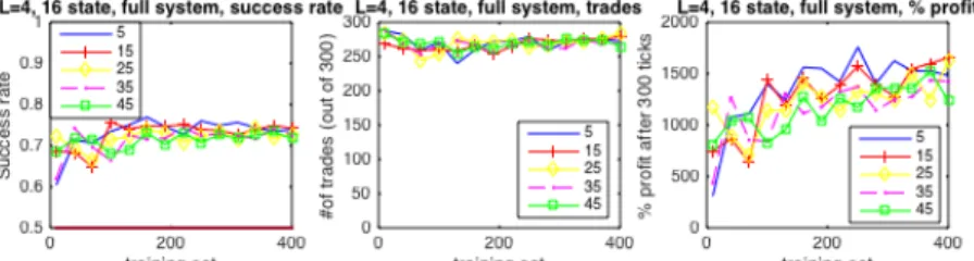
Figure 1 shows the corresponding three subfigures on different hist-num_neur combinations when predicting the full forward distribution, according to the trading strategy described in Section 3: with an increasing training set size, we quickly achieve over 70% success rate and the number of trades is around 270 with 𝜀 = 0.1, and as expected, the profit at the end of 300 trades increases exponentially with the success rate.

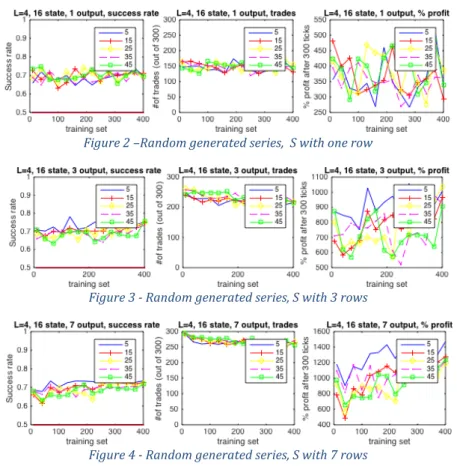
Figure 2 shows results using an S matrix with one row. As expected in the case of this specific S matrix, the number of trades is around 150, or 50%. Success rate is around 70% regardless of the number of neurons used, and the total profit after 300 is close to 400%. Increasing the size of the S matrix to three rows gives results shown in Figure 3. Here some clear trends emerge, namely: (i) smaller networks have a higher success rate, but make fewer trades, and (ii) with an increasing training set size, success rates saturate quickly. With matrix S having more rows, the number of trades increases to around 220, getting close to 75%.

As a conclusion, the smallest network gives the highest profit after 300 ticks, on average around 900%. Results, when using a matrix S with seven rows, are presented in Figure 4, which looks similar to the three row case, but the number of trades has now increased above 260, or 87% which is also in line with expectations. The overall profit after 300 ticks doubled to around 1300%.

These results demonstrate the applicability of the theory to randomly generated time series, and give us a good sense of how networks with various parameters perform. It also shows that the reduced complexity system requires a smaller training set than the full complexity system, but does not perform better at larger training sets.

(8)

Figure 2 –Random generated series, S with one row

Figure 3 - Random generated series, S with 3 rows

Figure 4 - Random generated series, S with 7 rows

5.2. Performance on real stock data

Having investigated the performance of our algorithms on randomly generated datasets, we now use the method for trading on stock prices. We have downloaded 1-hour tick stock data from NASDAQ and NYSE between the 26^th of October, 2015, and the 30^th of May, 2016. We extracted the time series for all of the SP500 stocks, and generated a number of portfolios, each consisting of five different stocks.

We selected portfolios with only a small amount of movement in the mean; this is because our algorithms perform best when the time series takes its values on a large fraction of the price levels for any given time window. Thus due to the examples covering the whole state space we obtain a “rich” training set and the FFNN can successfully learn the forward distribution. If it is not the case, and the mean shifts, then after training we observe such input values that were not included in the training set, which results in poor generalization. For the same reason, we have restricted the training set sizes between 10 and 300.

Table 1 - Stocks and weights of the three portfolios

Portfolio 1 PRU OKE IP AMGN WDC

14.16 8.55 -0.36 15.3 -24.24

Portfolio 2 VLO TIF A CHD FL

18.87 -12.54 -1.58 7.88 11.16 Portfolio 3 NKE CHRW TROW FTR SCG

23.91 15.67 -19.31 -13.13 -7.11

(9)

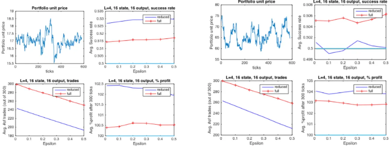
First, we evaluate Portfolio 1; results are shown in Figure 4, here we only evaluate the strategy with an S matrix that has seven rows (exhibiting the best performance on generated data). Trading begins at the

400^th tick mark, and continues to the 700^th tick. We compare the full complexity, forward-distribution estimation algorithm, shown in Figure 5, to the reduced complexity one, shown in Figure 6, both at 𝜀 = 0.1. As expected, the success rate is only a few percent points above 50%, but consistently so, and given the large number of trades, after 300 ticks, our profit is around 102-105%. The profit with a buy-and-hold strategy (buy at the first tick sell at 300) is 98% (2% loss), though.

Clearly, the full complexity system carries out more trades, but with a lower success rate compared to the reduced complexity system. In the reduced complexity case, we also observe a decreasing number of trades as the length of the training set is increased, which is likely due to overfitting and the changing statistical properties of the time series.

Figure 5 – Portfolio 1, full system

(10)

Figure 6 Portfolio 1, S with 7 rows

Figure 7 shows the averaged results of the full complexity system compared to the averaged results of the reduced complexity system, while changing epsilon, the threshold for trading. As epsilon increases, the number of trades falls rapidly, but the average success rate improves, showing that the outputs of the neural networks indeed represent the probability of increase or decrease.

Furthermore, the loss from incorrect trading predictions also decreases, leading to a slight overall increase in the profit at the end of 300 ticks. The reduced system clearly performs much better than the full complexity system. Figure 8 shows matching figures for portfolios 2 and 3, underlining the efficiency of the reduced complexity system. Notably, for portfolio 3, the success rate is worse for the reduced complexity system, but the overall profit is higher, due to smaller losses when the wrong trading decision is made.

(11)

Figure 8 – Portfolio 2 and 3, varying epsilon

Finally, we introduce a new trading strategy in which we are concurrently running the predictive algorithm on all three portfolios described previously, and at each tick we trade with the one with the highest probability of increase or drop. Results are shown in Figure 9, which outperform all of the individual portfolios, making more than 290 out of 300 possible trades, achieving a higher success rate, and giving an average profit of 107.3%, or up to 115% is some cases.

Figure 9 – Concurrent trading strategy

6. Conclusions

In this paper, we have presented a neural network based Bayesian trading algorithm, predicting a time series by having a neural network learn the forward conditional probability distribution of state transitions, when the values are discretized. Recognizing one of the key limitations of the algorithm, we designed a complexity reduction scheme by developing a special coding technique that makes training viable even on shorter training sets. We have implemented this trading algorithm, and demonstrated that it can learn the distribution of a randomly generated time series, yielding successful trading decisions on them.

Then we tested the performance of the new method on real stock data from NASDAQ and NYSE. As demonstrated the method is profitable even on real data.

Furthermore, it has been pointed out that as far as the profit is concerned the system with low complexity encoding performs as well as the one with the orthogonal coding scheme.

Acknowledgements

The research reported here has been supported by Grant KAP15-062-1.1-ITK.

(12)

REFERENCES

[1] Hornik, K, Stinchcombe, M, White, H Multilayer Feedforward Networks are Universal Approximators. Neural Networks, VOL. 2, 1989, pp.359-366.

[2] Funahashi,K.I.On the Approximate Realization of Continuous Mappings by Neural Networks. Neural Networks, VOL. 2, 1989, pp.183-192.

[3] Haykin, S. Neural Network Theory: a Comprehensive Foundation, Prentice Hall, 1999.

[4] Anagnostopoulos, K.P., and Mamanis, G. (2011) The mean-variance cardinality constrained portfolio optimization problem: An experimental evaluation of five multiobjective evolutionary algorithms.. Expert Systems with Applications, 38:14208-14217

[5] Banerjee, O., El Ghaoui, L., d’Aspermont A. (2008) Model Selection Through Sparse Maximum Likelihood Estimation.

Journal of Machine Learning Research, 9: 485-516

[6] Box, G.E., Tiao, G.C. (1977) A canonical analysis of multiple time series. Biometrika 64(2), 355-365

[7] Chen, L., Aihara, K. (1995) Chaotic Simulated Annealing by a Neural Network Model with Transient Chaos Neural Networks 8(6) 915-930

[8] D’Aspermont, A, Banerjee, O., El Ghaoui, L.(2008) First-Order Methods for Sparce Covariance Selection. SIAM Journal on Matrix Analysis and its Applications, 30(1) 56-66

[9] D’Aspremont, A.(2011) Identifying small mean-reverting portfolios. Quantitative Finance, 11:3, 351-364

[10] Fama, E., French, K.(1988) Permanent and Temporary Components of Stock Prices. The Journal of Political Economy 96(2), 246-273

[11] Manzan, S. (2007) Nonlinear Mean Reversion in Stock Prices. Quantitative and Qualitative Analysis in Social Sciences, 1(3), 1-20

[12] Markowitz, H. (1952) Portfolio Selection. The Journal of Finance 7:1,77-91

Low complexity algorithmic trading by Feedforward Neural Networks