Motor imagery EEG classification using feedforward neural network ∗

(1)

Motor imagery EEG classification using feedforward neural network ^∗

Tamás Majoros

^a

, Stefan Oniga

^ab

, Yu Xie

^a

aIntelligent Embedded Systems Research Laboratory, Faculty of Informatics, University of Debrecen

majoros.tamas@inf.unideb.hu yu.xie@inf.unideb.hu oniga.istvan@inf.unideb.hu

bTechical University of Cluj-Napoca, North University Centre of Baia Mare

Submitted: December 21, 2020 Accepted: April 19, 2021 Published online: May 18, 2021

Abstract

Electroencephalography (EEG) is a complex voltage signal of the brain and its correct interpretation requires years of training. Modern machine- learning methods help us to extract information from EEG recordings and therefore several brain-computer interface (BCI) systems use them in clinical applications.

By processing the publicly available PhysioNet EEG dataset, we extracted information that could be used for training feedforward neural network to classify three types of activities performed by 109 volunteers. While volunteers were performing different activities, a BCI2000 system was recording their EEG signals from 64 electrodes. We used motor imagery runs where a target appeared on either the top or the bottom of a screen. The subject was instructed to imagine opening and closing either both his/her fists (if the target is on top) or both his/her feet (if the target is on the bottom) until the target disappears from the screen.

We used the EEGLAB Matlab toolbox for EEG signal processing and applied several feature extraction techniques. Then we evaluated the classification performance of feedforward, multilayer perceptron (MLP) networks

∗This work was supported by the construction EFOP-3.6.3-VEKOP-16-2017-00002. The project was supported by the European Union, co-financed by the European Social Fund.

doi: https://doi.org/10.33039/ami.2021.04.007 url: https://ami.uni-eszterhazy.hu

235

(2)

with different structures (number of layers, number of neurons). Achieved accuracy score for test data was 71.5%.

Keywords:Neural network, multilayer perceptron, classification, EEG, BCI

1. Introduction

During brain activity ionic current flow generates voltage fluctuations that can be measured on the scalp with electrodes. Measured signals (electroencephalogram, EEG) are quite complex and their correct interpretation demands expertise.

However, due to the great advances in machine learning science, machine learning techniques are increasingly used for interpreting EEG signals [3, 10].

A brain–computer interface (BCI) is a communication pathway between a brain and a computer. A possible application area is to perform certain physical effects with just brain waves, not using muscles. This can be helpful for people who are immobile, elderly or paralyzed, therefore these systems are widely used for clinical applications in both rehabilitation [2] and communication [8].

Motor imagery is the imagination of the movement of various body parts. It causes cortex activation and oscillations in the EEG, therefore it can be detected by the BCI device to infer a user’s intent. Accurate and sufficiently fast recognition of the activity to be performed is essential in developing such BCI applications.

Artificial neural networks (ANN) are integral parts of BCI systems in many cases. The goal of our work is to create a neural network that can be applied in BCI applications to recognize motor imagery activities. However, in order for these networks to perform well, they need many training examples.

Creating a database which is suitable for training neural networks requires a lot of volunteers, an advanced data collection system, and several months of work.

Fortunately, there are quite a few EEG databases that are publicly available. These were made for different purposes, for example for recognition of motor imagery, epileptic seizure, various brain lesions. To avoid the difficulties of creating our own database, we used such a publicly available database.

In recent years, a number of consumer-grade BCI devices have been developed that are allowed to use outside of clinical settings [9]. In the future we would like to use a neural network trained on a large, public database to recognize EEG signals recorded by our own BCI device.

2. PhysioNet EEG dataset

Researchers created numerous EEG datasets for various purposes and made them publicly available. Some of them are made to evaluate and study various health- related problems, such as epilepsy, autism or sleep disorders. Another common area of use is related to motor and motor imagery activities. One such dataset is the PhysioNet EEG dataset [4], which contains one- and two-minute EEG recordings from 109 volunteers.

(3)

Researchers used the BCI2000 software suite to record brain waves while subjects performed various tasks. 14 measurements were performed on all 109 volunteers, resulting in 1526 one- and two-minute data files. Two of the 14 measurements are baseline runs with eyes open and closed, these are one minute long. The re- maining 12 are two-minute runs: two motor and two motor imagery measurements, repeated three times. These activities are:

• A target appears on the left or right side of the screen. The volunteer closes the fist on that side.

• A target appears on the left or right side of the screen. The volunteer imagines closing the fist on that side.

• A target appears on the top or bottom side of the screen. The volunteer closes both fists or feet, respectively.

• A target appears on the top or bottom side of the screen. The volunteer imagines closing both fists or feet, respectively.

We used those motor imagery runs where a target appeared on the top or the bottom of a screen. The subjects imagined opening and closing either both fists (if the target is on top) or both feet (if the target is on the bottom). Subjects were given new tasks every four seconds.

The data are available in EDF+, which is a standard EEG data recording format [6]. It includes the use of standard electrode names and supports timestamped annotations. EEG data were recorded from 64 electrodes with a sampling frequency of 160 Hz. The 64 electrodes were placed on the scalp as per the international 10-10 system.

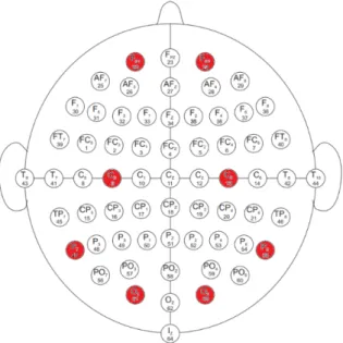
Figure 1. Placement of electrodes on the head.

(4)

Since we want to use the neural network trained on this dataset to process our own data in the future, it is important to use only those data that can be acquired by our own device too. Our device is an OpenBCI Ultracortex Mark IV headset with Cyton board. It has eight channels: C3, C4, Fp1, Fp2, P7, P8, O1 and O2, so only these channels were taken into account. The available electrodes in PhysioNet database are shown in Figure 1. The eight channels available on our device are marked in red.

3. Method

3.1. Data preprocessing

Electrophysiological signals, including EEG can be effectively processed in Matlab using the EEGLAB toolbox [1]. It provides a graphical user interface (GUI) allow- ing users to interactively process data. It supports various file formats, including EDF, and several data processing methods like independent component analysis (ICA) and time/frequency analysis (TFA).

The original scalp data is a matrix. Time course of the measured voltages on the channels are represented by the rows of the matrix. Since measurements are approximately two minutes long with 160 Hz sampling frequency, and eight channels are used, the size of the data matrix is 8×19920.

An additional three rows were added to the matrix to show which activity was being performed by the volunteer at the time of sampling. In each column, one of the three values is one and the other two are zeros according to the current activity (fists, feet, relax). These additional three rows extend the size of the matrix to 11×19920.

A frequently used data preprocessing step is the feature extraction from the raw data to make the applied machine learning model more effective. These features can be extracted from the wavelet, frequency, or time domain.

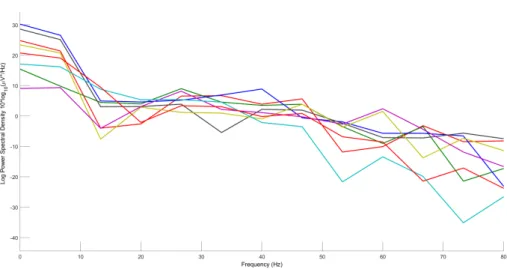
In the case of EEG signals, neural oscillations can be observed in the frequency domain. Time-series data can be transformed to the frequency domain using spectral methods. Figure 2 shows the distribution of the signal power over frequency for the first second of the first measurement of the first volunteer. To achieve this, power spectrum density (PSD) function was used.

The frequency components are often grouped into bands, these are the alpha, beta, gamma, delta and theta bands. The frequency limits of the bands are not precisely defined, the limits used are slightly different for different articles [5, 7, 11]. Ranges used by us are summarized in Table 1. Absolute power of the signal in the five frequency bands was also calculated. We used eight channels and five frequency bands, therefore we got 40 extra values for each time of sampling. These were also added to the data matrix to make them usable as inputs for the neural network.

(5)

Figure 2. Power spectral density of a one-second window.

Table 1. Bands and their frequency ranges.

Band Frequency range

Alpha 8-14 Hz

Beta 14-30 Hz

Gamma 30-80 Hz

Delta 1-4 Hz

Theta 4-8 Hz

To separate linearly mixed independent sources in EEG sensors, we performed independent component analysis (ICA). The result of the analysis is an invert- ible data decomposition. Several algorithms are provided by the EEGLAB. We used the Infomax because of its efficiency. In EEGLAB the Infomax algorithm re- turns two matrices, a data sphering matrix (icasphere) and the ICA weight matrix (icaweights) [1]. Their product is the unmixing matrix:

𝑈 =𝑖𝑐𝑎𝑤𝑒𝑖𝑔ℎ𝑡𝑠×𝑖𝑐𝑎𝑠𝑝ℎ𝑒𝑟𝑒.

The product of the unmixing matrix and the raw data matrix is the activation matrix. Each row of this represents the time course of the activity of one component process spatially filtered from the raw data.

𝐴=𝑈×𝑟𝑎𝑤𝑑𝑎𝑡𝑎.

After the ICA decomposition, power values were calculated again and both the activation matrix and the power matrix were added to the data matrix. Fig- ure 3 shows the component map of the first measurement of the first subject. Eye artifacts can be clearly seen in EEG data.

(6)

Figure 3. Component map of the first measurement of the first volunteer.

3.2. Machine learning chain

The machine learning process involves several steps and can therefore be considered as a chain. In our case, these steps are the import of the raw data, preprocessing (including normalization, segmentation and feature extraction), neural network instantiation, training and test.

The data from the sensors form a continuous stream of discrete values. Training the neural network with raw sensor data typically does not give adequate classification performance. As a result, some kind of data preprocessing is inevitable to improve it. As a first step, we used segmentation, which is the division of the available data into smaller units (windows).

Finding the appropriate window size is the main challenge in this task. If it is too small, it may not provide enough information about the performed activity, causing lower classification accuracy. Otherwise it may cover more than one activity in one window and causes increased latency. We tried numerous FFT window sizes for power spectral density calculation. Windows were overlapping, at each sample the window consisted the current sample and the previous N-1 samples. Then the order of the columns was shuffled randomly in the data matrix.

We used feedforward, multi-layer perceptron (MLP) networks and compared different architectures to improve accuracy. In all cases, the Levenberg-Marquardt backpropagation training method was used with the same training data: a two- minute motor imagery measurement from the first subject. Initial weights came from a normal Gaussian distribution, epoch limit was 1000 cycles. Number of hidden layers was one or two with 20 or 60 neurons. Activation functions were log- sigmoid and hyperbolic tangent sigmoid. Since there were three different classes, the number of neurons in the output layer was also three and its activation function was linear.

Best results were achieved with the two-layer network using log-sigmoid function

(7)

in both hidden layers as shown in Figure 4, thus in further work this was the applied architecture.

Figure 4. Structure of the applied neural network.

4. Results

Initially, we worked with a smaller amount of data (one two-minute measurement) and the indicator used to evaluate the performance of the network was accuracy.

It gives the ratio of the correct predictions to total predictions:

Accuracy=Number of correct predictions Total number of predictions .

Using only the raw data (8 inputs), without any features, the classification accuracy on test data was 56.2%. By adding band powers too (calculated with 0.5 second window size), using 48 inputs, accuracy was significantly better, 91.5%.

Using only the 40 power values did not cause a change in the classification performance, so in order to reduce training time, raw data were no longer used.

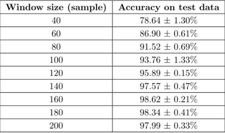
To find an appropriate FFT window size for band power calculation, neural network was trained using various windows sizes. Training and test with the data of a two-minute measurement from one subject were repeated five times to decrease statistical uncertainty. Applied neural network was the 2-layer MLP with 20-20 neurons in the hidden layers. Accuracy and its standard deviation on training and test data for different window sizes are summarized in Table 2.

Table 2. Accuracy for different window sizes.

Window size (sample) Accuracy on test data

40 78.64 ± 1.30%

60 86.90 ± 0.61%

80 91.52 ± 0.69%

100 93.76 ± 1.33%

120 95.89 ± 0.15%

140 97.57 ± 0.47%

160 98.62 ± 0.21%

180 98.34 ± 0.41%

200 97.99 ± 0.33%

(8)

Based on the above results, a window size of 160 samples is a reasonable choice, as it contains enough information about the activity performed, but does not yet cause too much latency in the case of real-time data processing, since whenever the target appears on the screen, in approximately one second we are able to determine from the EEG signal what the subject sees.

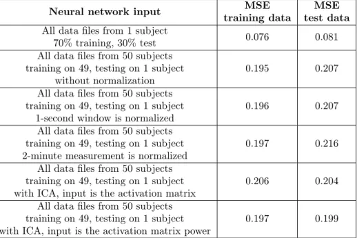
The same 2-layer MLP with 20-20 neurons in the hidden layers was tested on another same-type data file from the same volunteer. Classification accuracy was only 42.1%. To improve accuracy, we merged the three same-type data matrix from the same subject to one bigger matrix. 70% of this data was used for training and the rest for testing. A mean squared error (MSE) of 0.076 was achieved for the training and 0.081 for the test data.

As a new approach, we processed data from 50 subjects using the leave-one-out method: data from 49 subjects were used for training, the last one for testing.

MSE was 0.195 for the training and 0.207 for the test data.

In order to improve the classification accuracy of the neural network, we normalized the input data. Two different methods were used: in the first case, the raw data of the given one-second window were normalized before the power calculation, while in the second case, the data of the entire two-minute measurement were. MSE values were 0.196 (training) and 0.207 (test) in the first case, 0.197 (training) and 0.216 (test) for the second case. Normalization did not affect neural network performance in terms of MSE, so this was no longer used.

Table 3. Achieved MSE for the different experiments.

Neural network input MSE

training data MSE test data All data files from 1 subject

70% training, 30% test 0.076 0.081

All data files from 50 subjects training on 49, testing on 1 subject

without normalization 0.195 0.207

1-second window is normalized 0.196 0.207

2-minute measurement is normalized 0.197 0.216 All data files from 50 subjects

training on 49, testing on 1 subject

with ICA, input is the activation matrix 0.206 0.204 All data files from 50 subjects

training on 49, testing on 1 subject

with ICA, input is the activation matrix power 0.197 0.199 Furthermore in order to improve the performance, we applied independent com-

(9)

ponent analysis (ICA) on raw data and the activation matrix served as input for the neural network. We got 0.206 MSE value for training and 0.204 for test data.

Then we calculated the power values of the activation matrix and used the 40 power values as inputs. MSE values were 0.197 and 0.199 for training and test data, respectively. Results are summarized in Table 3.

In terms of classification accuracy, we found that the network recognized relaxation task with much greater accuracy than motor imagery tasks. This is because the data set was unbalanced, with much more data available for the relaxation task. To avoid this, we performed a balancing of the data set so that the same number of samples was available for all three activities. In addition, we increased the number of neurons to 60-60 in the hidden layers. The data of 10 volunteers were used, divided into two parts: 70% training, 30% test data. Training time on our computer (CPU: Intel Core i7-4790, RAM: 8 GB) was around 100 hours, accuracy for test data was 71.5%.

5. Conclusions

In this paper we proposed a multilayer perceptron (MLP) neural network approach for motor imagery task recognition from EEG data. In the longer term, the aim of our research is to use a neural network trained on a large dataset to analyze data recorded by our own device. Accordingly we used a publicly available dataset and tried to recognize the motor imagery activities of the subjects. We applied several data preprocessing methods and examined their effects on the performance of the neural network.

Our results demonstrated the importance of data preprocessing, and its effects on the classification performance of a neural network. However, it also showed that MLP might not be the best choice for EEG classification, as the classification accuracy score achieved is not high enough. J. Wang et al. [13] showed that compared with MLP, SVM and linear discriminant analysis (LDA), convolutional neural network (CNN) can provide better EEG signal classification performance. Tang at al.

[12] applied conventional classification methods, such as power + support vector machine (SVM), CSP+ SVM, autoregression (AR) + SVM and compared them with deep CNN in motor imagery EEG classification. The performance of CNN was better than the other three methods. Our preliminary results using CNN also show a much better accuracy score which is over 90%.

References

[1] A. Delorme,S. Makeig:EEGLAB: an open source toolbox for analysis of single-trial EEG dynamics including independent component analysis, Journal of Neuroscience Methods 134.1 (2004), pp. 9–21,

doi:https://doi.org/10.1016/j.jneumeth.2003.10.009.

(10)

[2] L. van Dokkum,T. Ward,I. Laffont:Brain computer interfaces for neurorehabilitation – its current status as a rehabilitation strategy post-stroke, Annals of Physical and Rehabil- itation Medicine 58.1 (2015), pp. 3–8,

doi:https://doi.org/10.1016/j.rehab.2014.09.016.

[3] L. A. Gemein, R. T. Schirrmeister, P. Chrabąszcz, D. Wilson, J. Boedecker, A. Schulze-Bonhage,F. Hutter,T. Ball:Machine-learning-based diagnostics of EEG pathology, NeuroImage 220 (2020), p. 117021,

doi:https://doi.org/10.1016/j.neuroimage.2020.117021.

[4] A. L. Goldberger,L. A. Amaral,L. Glass,J. M. Hausdorff,P. C. Ivanov,R. G.

Mark,J. E. Mietus,G. B. Moody,C. K. Peng,H. E. Stanley:PhysioBank, Phys- ioToolkit, and PhysioNet: components of a new research resource for complex physiologic signals, Circulation 101.23 (2000), pp. 215–220,

doi:https://doi.org/10.1161/01.CIR.101.23.e215.

[5] I. S. Isa,B. S. Zainuddin,Z. Hussain,S. N. Sulaiman:Preliminary Study on Analyzing EEG Alpha Brainwave Signal Activities Based on Visual Stimulation, Procedia Computer Science 42 (2014), pp. 85–920,

doi:https://doi.org/10.1016/j.procs.2014.11.037.

[6] B. Kemp,J. Olivan:European data format ‘plus’ (EDF+), an EDF alike standard format for the exchange of physiological data, Clinical Neurophysiology 114.9 (2003), pp. 1755–1761, doi:https://doi.org/10.1016/S1388-2457(03)00123-8.

[7] D. Kučikien ˙e,R. Praninskien ˙e:The impact of music on the bioelectrical oscillations of the brain, Acta medica Lituanica 25.2 (2018), pp. 101–106,

doi:https://doi.org/10.6001/actamedica.v25i2.3763.

[8] I. Lazarou,S. Nikolopoulos,P. C. Petrantonakis,I. Kompatsiaris,M. Tsolaki:

EEG-Based Brain-Computer Interfaces for Communication and Rehabilitation of People with Motor Impairment: A Novel Approach of the 21 st Century, Frontiers in human neuroscience 12 (2018),

doi:https://doi.org/10.3389/fnhum.2018.00014.

[9] R. Maskeliunas,R. Damasevicius,I. Martisius,M. Vasiljevas:Consumer grade EEG devices: are they usable for control tasks?, PeerJ 4 (2016),

doi:https://doi.org/10.7717/peerj.1746.

[10] Y. Roy,H. Banville,I. Albuquerque,A. Gramfort,T. H. Falk,J. Faubert:Deep learning-based electroencephalography analysis: a systematic review, Journal of Neural En- gineering 16.5 (2019),

doi:https://doi.org/10.1088/1741-2552/ab260c.

[11] J. Suto,S. Oniga,P. P. Sitar:Music stimuli recognition from electroencephalogram signal with machine learning, in: 2018 7th International Conference on Computers Communications and Control (ICCCC), 2018, pp. 260–264,

doi:https://doi.org/10.1109/ICCCC.2018.8390468.

[12] Z. Tang,C. Li,S. Sun:Single-trial EEG classification of motor imagery using deep convolutional neural networks, Optik - International Journal for Light and Electron Optics 130 (2017), pp. 11–18,

doi:https://doi.org/10.1016/j.ijleo.2016.10.117.

[13] J. Wang,G. Yu,L. Zhong,W. Chen,Y. Sun:Classification of EEG signal using convolutional neural networks, in: 2019 14th IEEE Conference on Industrial Electronics and Applications (ICIEA), 2019, pp. 1694–1698,

doi:https://doi.org/10.1109/ICIEA.2019.8834381.