calibration to a neural network based monocular collision avoidance system on a
UAV ?
Antal Hiba,∗,∗∗ Rita Aleksziev,∗,∗∗ Kopp´any P´azm´an,∗,∗∗∗
P´eter Bauer,∗,∗∗ Andr´as Bencz´ur,∗,∗∗ Akos Zar´´ andy∗,∗∗
B´alint Dar´oczy∗,∗∗
∗ Institute for Computer Science and Control, Hungarian Academy of Sciences, Budapest, Hungary
∗∗ Research Center of Vehicle Industry, Sz´echenyi Istv´an University, Gyor, Hungary
∗∗∗ P´azm´any P´eter Catholic University, Budapest, Hungary
Abstract:Contextual calibration for object detection is a technique where a pretrained network collects attractive false positives during a calibration phase and use this calibration data for further training. This paper investigates the applicability of this method to a vision based on- board sense and avoid system, which requires intruder aircraft detection in camera images.
Various landscape and sky backgrounds were generated by Unreal4 3D engine for calibration tests. Contextual calibration is a promising candidate for handling extreme situations which are not covered well in the training data.
Keywords:Learning, adaptation and evaluation; Aerospace; Robotics and autonomous systems 1. INTRODUCTION
Sense and avoid (SAA) capability is a crucial ability for the future unmanned aerial vehicles (UAVs). It is vital to integrate civilian and governmental UAVs into the com- mon airspace according to EU (2013) for example. At the highest level of integration Airborne Sense and Avoid (AB- SAA) systems are required to guarantee airspace safety Dempsey (2010).
In this field the most critical question is the case of non- cooperative SAA. However, in the case of small UAVs the size, weight and power consumption of the on-board SAA system should be minimal.
There are commercial stereo camera solutions for quad- copters with smaller range (DJI Mavic Air 25m range), and small sized but relatively expensive complete radar solu- tions (Fortem TrueView Radar). Monocular vision-based approach can be cost and weight effective therefore espe- cially good for small fixed-wing UAVs. Recent work of our lab Bauer et al. (2019) presents the theory of evaluation of the collision situation in three dimension (3D) estimating time to closest point of approach (TTCPA), horizontal and vertical closest point of approach (CPA) and the direction of the CPA (βCP A) as it is not necessarily perpendicular to own aircraft forward body axis. The evaluation technique assumes straight flight trajectories in 3D.
? Research is supported by 2018-1.2.1-NKP-00008: Exploring the Mathematical Foundations of Artificial Intelligence and by MTA Premium Postdoctoral Grant 2018. This paper was also supported by the J´anos Bolyai Research Scholarship of the Hungarian Academy of Sciences and the Higher Education Institutional Excellence Program.
All vision-based collision avoidance methods require ro- bust detection and tracking of the intruder in the image Fasano et al. (2014); Rozantsev et al. (2015, 2017). The problem is still unsolved and sensor fusion techniques are applied to improve robustness. The cooperation of the UAVs, which is a special form of sensor fusion, can efficiently enhance the detection Opromolla et al. (2018) .
“Deep” learning methods can be fine tuned for matching, Chen et al. (2017) and for trajectory planning as in Khan and Hebert (2018).
Camera sensors are cheap and they provide a large amount of information at high refresh rate, however, on-board computation is challenging. Neural networks with appro- priate training data give the best solution for most image processing tasks. Furthermore, these networks can be in- ferred on a small sized low power ’edge’ hardware thus they can be applied in small UAV SAA systems.
Ideal training data covers all the possible cases with the same possibility as they appear in real situations (no oversampling of a case). Acquiring real flight data with close encounters is a very hard job, and it is necessary to get data in different seasons and landscapes with different sky backgrounds. Photorealistic simulator environments Shah et al. (2017) can provide this variability, but we always seek new data. Close encounters are rare events, and we can ensure in some situations that we can not see any intruders. For instance the operator can see that one direction is safe during takeoff and can let the drone fly towards that direction for a while to collect data, which has only negative samples (all possible region of interest- ROI has no intruder). This data corresponds to the actual
situation (landscape, sky) and can be used to further train the network on-board to have better performance on the current flight. We call this process contextual calibration, and this paper aims to investigate the effect and applicability of this approach in the case of monocular UAV SAA systems.
2. MONOCULAR COLLISION AVOIDANCE SYSTEM 2.1 Test UAVs and main concept
Real flight tests are conducted with two UAVs on an airfield near Budapest (Hungary) Zsedrovits et al. (2016).
The own aircraft is a large 3.5m wingspan, about 10-12 kg twin-engine UAV called Sindy which is developed in our institute to carry experimental payloads such as the Sense
& Avoid system (for details and building instructions - as it is an open source project - see SZTAKI (2014)).
The intruder UAV is the E-flite Ultrastick 25e which is a small 1.27m wingspan 1.5-2 kg single engine drone. The small size of the intruder makes detection and decision about the collision extremely difficult.
During a flight test the two aircrafts are heading towards each other with small vertical separation and varying horizontal separation (flight paths are parallel). Time to CPA (TTCPA) is also estimated and CPA is a signed value which helps maneuver planning. The system triggers evasion maneuver if the absolute value of the calculated CPA is smaller than the threshold at a given decision time.
We set up a Closest Point of Approach (CPA) threshold approx. 15 which means 15 times the unknown size of the intruder (in this case 15 m). The general 3D straight trajectory version has not been flight tested yet.
Fig. 1. Main components of the on-board sense and avoid system: Flight Control Computer, the Camera sensors and the Nvidia Jetson TX1 payload computer for image processing and decision making.
2.2 On-board Vision System
Figure 1 summarizes the modules of the on-board vision system. The payload computer consists of a quad-core ARM Cortex-A57, 4GB LPDDR4 and 256-core Maxwell GPU and consumes less than 20 W. We have two Basler HD cameras and the system should detect and track intruders against sky background. Sky-Ground separation is not used in this article because the neural network could distinguish sky intruders from ground objects. Candidate objects are proposed by a preprocessor which is a special blob detection. The key component is the classifier which assigns intruder confidence to each ROI. In Figure 2 we
show only 10 candidate ROIs which have the highest intruder confidence. The filtering proposes a hundred candidates on average per frame. Our main contribution is based on the idea to enhance the classifier with contextual calibration at the beginning of an autonomous flight.
Fig. 2. The 10 highest response candidate ROI (green) the ground truth ROI (blue)
3. CONTEXTUAL CALIBRATION AND OBJECT DETECTION
In traditional object detection the models are either “shal- low” or in case of ensemble models hierarchical yet “shal- low” in the sense of inner representation Felzenszwalb et al.
(2008); Benenson et al. (2012). In many cases the lack of learnable patch filters and rigid feature extraction with computationally unfeasable solutions for scaling and spa- tial segmentation result underperforming in complex mod- els, each with its own distinctive advantages. For example deformable parts models Felzenszwalb et al. (2010) scan the whole image on different scales with various sliding windows and the classifier part evaluates on every single window while the model is capable of learning from a small data set. In comparison, Benenson et al. (2012) filter out the majority of sliding windows with a simple model and only classify the remaining patches with a more accurate although computationally more expensive model achieving under 10ms performance on GPGPUs.
Another solution would be to replace rigid feature ex- traction and learn them on the fly together with the classifier given that the available training data is suffi- cient for “deep” models. The common element of various regions with convolutional neural network features (R- CNN)models are the proposal subnetwork to identify can- didate positions and bounding boxes Girshick (2015);Ren et al. (2015) and He et al. (2017). Since the models contain enormous amount of parameters they often utilized previ- ously learned convolutional maps (e.g. VGG-net Simonyan and Zisserman (2014);Huh et al. (2016)) to avoid lack of labeled data. The main disadvantage of the R-CNN method is inference performance. More recent methods offer near real-time inference on capable mobile devices though training is still considered cumbersome Liu et al.
(2016);Redmon et al. (2016) and Redmon and Farhadi (2018) on devices as Tegra X1 with limited memory and computational resources.
In this work, we benefit from the specific model adaptation problem by treating it as a feature-based transfer learn- 2
ing problem with available negative auxiliary data at the beginning of the flight. The main idea of transfer learning methods is to change the underlying distribution estimated on a source data set to fit target distribution. There are instance-based and feature-based transfer learning meth- ods Hu et al. (2015). Former methods transform the source instance to the target domain while feature-based methods transfer the underlying feature space learned on the source to have similar distribution on the target domain. An in- teresting model was proposed in Long et al. (2017) to select important convolutional features for domain adaptation in visual recognition problems. Our problem is specific in two ways since we do not assume similar distributions on the target and source domain and we are highly constrained in time and data to learn the appropriate feature map almost in an instance. The closest results to our model are Shi et al. (2017) where the authors use an auxiliary data set with uncorrelated labeling to localize objects and Cao et al. (2018) where target labels are partially available.
Both method treat the available data as unlabeled or negative sample.
3.1 Proposed model
After preprocessing individual frames the convolutional neural network ranks the candidate patches to identify intruders. We built a feed-forward network with three hid- den layers shown in Fig. 3 and optimized the parameters with Adam Kingma and Ba (2014). In comparison to more general setups we assume simple objects as intruders in an environment with high variability. The crucial advantage of the small sized model is high inference performance at the cost of complexity and detection quality. Since the environment is not changing fast or at a significant rate we can assume similar background variability during short flights. This gives us the opportunity to fine tune our existing model to overcome the quality issues. Arguably the inference performance is highly constrained by capa- bilities of the existing hardware and will disappear in the future but the background variability is data dependent.
Therefore we focus on the unknown background problem with a very general idea in case of UAVs.
Fig. 3. Intruder classifier model based on filtered patches and a convolutional neural network.
4. RESULTS
In the case of contextual calibration we assume that we have a pretrained neural network for intruder ROI classification and we expose a novel situation to the system which has some changes compared to the training data.
To mimic this setup we created simulated flights in four different landscape environments with three different skies in Unreal4 Engine with AirSim plugin (Fig. 5).
Beyond our simulated data we also use the videos of Rozantsev et al. (2015) referred as CVPR data. Figure 4
gives an overview of the model generation to compare base models to the calibrated ones. Each flight starts with an arc to collect calibration data and it is followed by a straight trajectory phase when an intruder UAV approaches. For each frame of the calibration arc the candidates of the preprocessor are given to the base network and the ROIs with the highest confidence are added to the calibration data set as negative sample.
Positive intruder samples of the calibration data are chosen randomly from the training data of the base network i.e.
calibration optimize for rejecting the most attractive false positives extracted from current situation while retain correct classification of previously seen intruders.
Fig. 4. Model generation from a flight. For each flight we have three pairs of base and calibrated neural networks. The base models are trained on cvpr data or a subset of our data set with leaving out the cor- responding landscape or sky type. Calibration starts from the base network and further trains it utilizing the calibration data of the current flight. Because of the random nature of training we reproduce each base network five times.
Fig. 5. Example images of calibration phase: Snowy moun- tain landscape with clouds v2, Mountain landscape with clouds v1, Desert landscape with clear sky and Afghan landscape with clear sky. The 4 different landscapes and 3 different sky setups results 12 pos- sible combinations where each has 5 different flight paths (main angle) thus we have 60 test flights.
3
4.1 Connection to real flight
During the calibration phase the system uses the base network to collect the negative samples with the highest intruder confidence, however, we need to be sure that there is no intruder. If an intruder does appear in the calibration data, the calibrated network may learn that it is not an intruder. After take off, the operator can choose a direction with no flying object, and let the system fly towards that direction for at least 30 seconds. Our Nvidia jetson TX1 system has 5 FPS refresh rate which results 150 processed calibration images, and the UAV took approximately 500 m assuming that the operator aims for low speed during calibration.
While the system calibrate the network, the SAA system is ’blind’ due lack of processing power. Edge hardware solutions are not designed to run training on them because both manufacturers and software communities assume that the training phase will take place on a high perfor- mance desktop or a cloud service and low-power hardware systems are only infer. Using cloud service for calibration training is possible but the aircraft has to communicate both calibration data and network description. Our simple neural network can be trained on-board with TensorFlow 1.10 1. A 2 epoch (100 iterations of small batches) cali- bration takes 14 seconds which is mostly initialization as a 30 epoch training lasts 25 seconds. Before calibration the model will freeze and reload itself in TensorRT2 taking additional tens of seconds. During this stage the operator can take circles or even land. After calibration the system can start its autonomous flight.
4.2 The effect of contextual calibration
We can see contextual calibration as a transfer learning problem with available negative data from the destination distribution (landscape and sky case of UE4-based SAA simulation). We have three main source distributions:
CVPR data, own SAA data without the corresponding Landscape type, or the SAA data excluding the sky type of the given flight. The CVPR data includes various situations and quality varies more from the destination than the rest two sources which are coming from the same simulated environment.
We measured the quality of detection with Receiver Oper- ating Characteristics (ROC) Tan et al. (2013) and normal- ized Discounted Cumulative Gain (nDCG) J¨arvelin and Kek¨al¨ainen (2002) due to their threshold independence property. Both rank candidate patches according to con- tinuous prediction of the network. The main difference is that Area Under Curve value of ROC (AUC) penalize patches uniformly while nDCG decay logarithmic.
Table 1 and 3 show that base networks of CVPR has worse distinctive power than the base networks trained on subsets of SAA data. After five epochs on the CVPR data base networks (Table 2) underperform compared to two epoch based networks due specialization to the CVPR data with further training.
1 https://www.tensorflow.org
2 https://developer.nvidia.com/tensorrt
Table 1. Average AUC of ROI classification on each flight. Baselines are trained on CVPR
data for 2 epochs.
Landsape/Sky Base it10 it50 Afghan/all 0.8303 0.8177 0.8286
Desert/all 0.8182 0.8322 0.8523 Mountain/all 0.7370 0.7967 0.8476 Snowy/all 0.7222 0.7283 0.7284 all/Clear 0.7738 0.7915 0.8062 all/Cloud1 0.7776 0.7904 0.8040 all/Cloud2 0.7793 0.7993 0.8324 all/all 0.7769 0.7937 0.8142
Table 2. Average AUC of ROI classification on each flight. Baselines are trained on CVPR
data for 5 epochs.
Landsape/Sky Base it10 it50 Afghan/all 0.8210 0.8297 0.8367
Desert/all 0.7940 0.8295 0.8519 Mountain/all 0.6600 0.7635 0.7821 Snowy/all 0.6918 0.6861 0.6877
all/Clear 0.7420 0.7804 0.7879 all/Cloud1 0.7294 0.7698 0.7804 all/Cloud2 0.7537 0.7815 0.8004 all/all 0.7417 0.7772 0.7896
During calibration we used 20 as mini batch size. We measured calibrated network performance after 10 (we will refer the network as it10) and 50 (it50) iterations i.e. either 100 or 500 patches of the most attractive false positives were used for calibration. it50 calibrated networks per- formed better almost in all cases in comparison to it10.
For the CVPR base networks calibration has significant positive effect which can be seen in Figure 6.
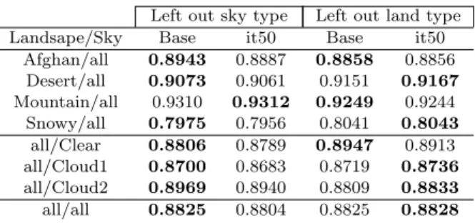
Table 3. Average AUC of ROI classification on each flight. Baselines are trained on SAA with
appropriate training subsets for 2 epochs.
Left out sky type Left out land type
Landsape/Sky Base it50 Base it50
Afghan/all 0.8943 0.8887 0.8858 0.8856 Desert/all 0.9073 0.9061 0.9151 0.9167 Mountain/all 0.9310 0.9312 0.9249 0.9244
Snowy/all 0.7975 0.7956 0.8041 0.8043 all/Clear 0.8806 0.8789 0.8947 0.8913 all/Cloud1 0.8700 0.8683 0.8719 0.8736 all/Cloud2 0.8969 0.8940 0.8809 0.8833 all/all 0.8825 0.8804 0.8825 0.8828
Table 3 contains the AUC results of the calibrated SAA base networks show no significant change in performance (Figure 7) albeit the base networks performed well on an unseen sky or land type.
In each frame we have plenty of candidates extracted from the preprocessor. In some cases the intruder overlaps several patches as seen in Fig. 2. We argue that in such a particular case the nDCG compare the performance of networks better than AUC as every part of the intruder ought to be detected. Worth to mention that while the AUC values are slightly worse for the calibrated networks, the nDCG@10 measures better ranking as seen in Table 4.
nDCG improvement suggests that even a well performing base network can benefit from contextual calibration.
4
Fig. 6. Histogram of AUC differences for cvpr 2 epoch baseline NN calibrated for 50 iterations (500 samples).
Fig. 7. Histogram of AUC differences for SAA 2 epoch baseline NN calibrated for 50 iterations (500 samples).
The corresponding sky or landscape types were left out from training data of the baseline NN.
Table 4. Average nDCG@10 of ROI classifica- tion on each flight. Baselines are trained on SAA with appropriate training subsets for two
epochs.
Left out sky type Left out land type
Landsape/Sky Base it50 Base it50
Afghan/all 0.9610 0.9625 0.9717 0.9713 Desert/all 0.9677 0.9717 0.9801 0.9814 Mountain/all 0.9544 0.9585 0.9508 0.9535 Snowy/all 0.8014 0.8039 0.8599 0.8700 all/Clear 0.8392 0.8395 0.8899 0.8949 all/Cloud1 0.9537 0.9619 0.9719 0.9732 all/Cloud2 0.9704 0.9710 0.9601 0.9641 all/all 0.9211 0.9241 0.9406 0.9440
5. CONCLUSIONS
In this paper we discussed the basic applicability ques- tions in case of contextual calibration for vision based SAA systems. The hardware and software components are available for on-board training for small networks, the main limiting factor is on-board memory. We have found that a network with good generalization capability can be efficiently tuned with contextual calibration if the use case has large difference from the training data, however,
in these cases further training data collection is inevitable for safe usage. A surprising remark that the calibration did not degrade the AUC performance in cases where the dif- ference from training data is less significant. Furthermore, the most relevant nDCG value became slightly better after calibration. In current form we do not recommend to use contextual calibration in machine vision systems because further investigation is required. Especially the change of the weights in the base network should be monitored as well as the performance change on the training data set.
With further investigation, we hope that contextual cali- bration can enhance robustness of machine vision systems against problems in rare situations.
REFERENCES
Bauer, P., Hiba, A., Bokor, J., and Zarandy, A. (2019).
Three dimensional intruder closest point of approach estimation based-on monocular image parameters in aircraft sense and avoid. Journal of Intelligent
& Robotic Systems, 93(1), 261–276. doi:10.1007/
s10846-018-0816-6.
Benenson, R., Mathias, M., Timofte, R., and Van Gool, L.
(2012). Pedestrian detection at 100 frames per second.
InComputer Vision and Pattern Recognition (CVPR), 2012 IEEE Conference on, 2903–2910. IEEE.
Cao, Z., Long, M., Wang, J., and Jordan, M.I. (2018).
Partial transfer learning with selective adversarial net- works. In The IEEE Conference on Computer Vision and Pattern Recognition (CVPR).
Chen, Y., Liu, L., Gong, Z., and Zhong, P. (2017). Learn- ing cnn to pair uav video image patches. IEEE Journal of Selected Topics in Applied Earth Observations and Remote Sensing, 10(12), 5752–5768.
Dempsey, M. (2010). U.s. army unmanned aircraft systems roadmap 2010-2035. Technical report, U.S. Army UAS Center of Excellence.
EU (2013). Roadmap for the integration of civil Remotely- Piloted Aircraft Systems into the European Aviation System. Technical report, European RPAS Steering Group.
Fasano, G., Accardo, D., Tirri, A.E., Moccia, A., and De Lellis, E. (2014). Morphological filtering and target tracking for vision-based uas sense and avoid. In Un- manned Aircraft Systems (ICUAS), 2014 International Conference on, 430–440. IEEE.
Felzenszwalb, P., McAllester, D., and Ramanan, D. (2008).
A discriminatively trained, multiscale, deformable part model. In Computer Vision and Pattern Recognition, 2008. CVPR 2008. IEEE Conference on, 1–8. IEEE.
Felzenszwalb, P.F., Girshick, R.B., McAllester, D., and Ramanan, D. (2010). Object detection with discrimina- tively trained part-based models.IEEE transactions on pattern analysis and machine intelligence, 32(9), 1627–
1645.
Girshick, R. (2015). Fast r-cnn. InProceedings of the IEEE international conference on computer vision, 1440–1448.
He, K., Gkioxari, G., Doll´ar, P., and Girshick, R. (2017).
Mask r-cnn. In Computer Vision (ICCV), 2017 IEEE International Conference on, 2980–2988. IEEE.
Hu, J., Lu, J., and Tan, Y.P. (2015). Deep transfer metric learning. InThe IEEE Conference on Computer Vision and Pattern Recognition (CVPR).
5
Huh, M., Agrawal, P., and Efros, A.A. (2016). What makes imagenet good for transfer learning? arXiv preprint arXiv:1608.08614.
J¨arvelin, K. and Kek¨al¨ainen, J. (2002). Cumulated gain- based evaluation of ir techniques.ACM Transactions on Information Systems (TOIS), 20(4), 422–446.
Khan, A. and Hebert, M. (2018). Learning safe recovery trajectories with deep neural networks for unmanned aerial vehicles. In2018 IEEE Aerospace Conference, 1–
9. IEEE.
Kingma, D. and Ba, J. (2014). Adam: A method for stochastic optimization. arXiv preprint arXiv:1412.6980.
Liu, W., Anguelov, D., Erhan, D., Szegedy, C., Reed, S., Fu, C.Y., and Berg, A.C. (2016). Ssd: Single shot multibox detector. InEuropean conference on computer vision, 21–37. Springer.
Long, M., Zhu, H., Wang, J., and Jordan, M.I. (2017).
Deep transfer learning with joint adaptation networks.
InProceedings of the 34th International Conference on Machine Learning - Volume 70, ICML’17, 2208–2217.
JMLR.org. URL http://dl.acm.org/citation.cfm?
id=3305890.3305909.
Opromolla, R., Fasano, G., and Accardo, D. (2018). A vision-based approach to uav detection and tracking in cooperative applications. Sensors, 18(10), 3391.
Redmon, J., Divvala, S., Girshick, R., and Farhadi, A.
(2016). You only look once: Unified, real-time object detection. In Proceedings of the IEEE conference on computer vision and pattern recognition, 779–788.
Redmon, J. and Farhadi, A. (2018). Yolov3: An incremen- tal improvement. arXiv preprint arXiv:1804.02767.
Ren, S., He, K., Girshick, R., and Sun, J. (2015). Faster r-cnn: Towards real-time object detection with region proposal networks. In Advances in neural information processing systems, 91–99.
Rozantsev, A., Lepetit, V., and Fua, P. (2015). Flying objects detection from a single moving camera. InPro- ceedings of the IEEE Conference on Computer Vision and Pattern Recognition, 4128–4136.
Rozantsev, A., Lepetit, V., and Fua, P. (2017). Detecting flying objects using a single moving camera.IEEE trans- actions on pattern analysis and machine intelligence, 39(5), 879–892.
Shah, S., Dey, D., Lovett, C., and Kapoor, A. (2017).
Airsim: High-fidelity visual and physical simulation for autonomous vehicles. In Field and Service Robotics.
URLhttps://arxiv.org/abs/1705.05065.
Shi, Z., Siva, P., and Xiang, T. (2017). Transfer learning by ranking for weakly supervised object annotation. arXiv preprint arXiv:1705.00873.
Simonyan, K. and Zisserman, A. (2014). Very deep convolutional networks for large-scale image recognition.
arXiv preprint arXiv:1409.1556.
SZTAKI, M. (2014). Sindy test aircraft. URL http://
uav.sztaki.hu/\-sindy/\-home.html.
Tan, P.N., Steinbach, M., and Kumar, V. (2013). Data mining cluster analysis: basic concepts and algorithms.
Introduction to data mining.
Zsedrovits, T., Peter, P., Bauer, P., Pencz, B.J.M., Hiba, A., Gozse, I., Kisantal, M., Nemeth, M., Nagy, Z., Vanek, B., et al. (2016). Onboard visual sense and avoid system for small aircraft. IEEE Aerospace and
Electronic Systems Magazine, 31(9), 18–27.
6