Ensemble noisy label detection on MNIST ∗

(1)

Ensemble noisy label detection on MNIST ^∗

István Fazekas

^a

, Attila Barta

^b

, László Fórián

^b

aUniversity of Debrecen, Department of Applied Mathematics and Probability Theory fazekas.istvan@inf.unideb.hu

bUniversity of Debrecen, Doctoral School of Informatics barta.attila@inf.unideb.hu

forian.laszlo@inf.unideb.hu Submitted: January 18, 2021

Accepted: March 29, 2021 Published online: May 18, 2021

Abstract

In this paper machine learning methods are studied for classification data containing some misleading items. We use ensembles of known noise correction methods for preprocessing the training set. Preprocessing can be either relabeling or deleting items detected to have noisy labels. After preprocessing, usual convolutional networks are applied to the data. With preprocessing, the performance of very accurate convolutional networks can be further improved.

Keywords:Label noise, deep learning, classification AMS Subject Classification:68T07

1. Introduction

In recent years, deep neural networks have reached very impressive performance in the task of image classification. However, these models require very large datasets with labeled training examples, and such datasets are not always available. The labeling process is often very expensive, or it is very difficult even for experts in a particular field. That is what can lead to the use of databases with label noise, which contain incorrectly labeled instances. Therefore, it is important to examine

∗This work was supported by the construction EFOP-3.6.3-VEKOP-16-2017-00002. The project was supported by the European Union, co-financed by the European Social Fund.

doi: https://doi.org/10.33039/ami.2021.03.015 url: https://ami.uni-eszterhazy.hu

125

(2)

training on this kind of datasets. According to a widely accepted assumption, deep networks learn consistent, simple patterns in the beginning, and then it is followed by the learning of the harder examples with possibly incorrect labels [2]. So treating the label noise in the training set can lead to a better generalization ability instead of its overfitting to the wrong examples. A lot of studies address the noisy label problems, for example, [1] is an extensive survey of a broad range of the existing methods.

In this work we investigate the possibilities of improving a classifier (which is an ensemble of deep neural networks) by handling the label noise in the training dataset. We classify with an ensemble of convolutional neural networks (CNNs).

At the start, we train that ensemble on the original training dataset. Then we are going to apply a label noise cleansing technique on the training data. Finally, we take a CNN ensemble with the same structure as our original CNN ensemble, and train it on the new dataset gained after treating the label noise. We evaluate and compare the performance of the ensemble classifiers and draw conclusions.

As our main goal is to study label correcting neural networks for preprocessing purpose, so here we use only simple ensemble building methods. The effect of more sophisticated voting systems (see, e.g. [7]) on our two-phase classification method can be studied later.

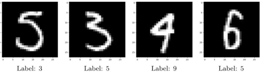
We conduct experiments on the MNIST dataset [6]. MNIST is a database of handwritten digits, it consists of images with28×28grayscale pixels. The size of the training set is 60 000examples and the test set has10 000samples. However, MNIST contains some misleading items. To support it, some examples that might be considered as mislabeled images can be seen on Figure 1.

Label: 3 Label: 5 Label: 9 Label: 5

Figure 1. Some misleading images in the MNIST dataset.

We shall consider the misleading items as inaccurately labelled ones so we can apply some known methods elaborated to handle noisy labels.

2. Methods to detect and correct label noise

In the beginning, let us define some notations. We denote vectors with bold (e.g.x) letters and matrices with capital (e.g.𝑋) letters. Specifically, 1corresponds to a vector of all-ones. In the 𝑐-dimensional space, the term of hard-label and soft-

(3)

label spaces are used, they are denoted by ℋ = {y : y ∈ {0,1}^𝑐,1^|y = 1} and 𝒮 = {y : y ∈ [0,1]^𝑐,1^|y = 1}, respectively. It is easy to see that ℋ contains one-hot vectors, and the elements of𝒮 are discrete probability distributions.

In an image classification problem with 𝑐 classes, we have a training set of 𝑛 images: 𝑋 ={x1,x2, . . . ,x𝑛}with the corresponding ground-truth

𝑌^𝐺𝑇 ={y^𝐺𝑇₁ ,y^𝐺𝑇₂ , . . . ,y^𝐺𝑇_𝑛 }

labels. y^𝐺𝑇_𝑖 ∈ ℋrepresents the class ofx𝑖with a1in the coordinate corresponding to that class.

Using a neural network with the cross entropy loss function, the model can be trained by minimizing

ℒ=−1 𝑛

∑︁𝑛

𝑖=1

∑︁𝑐

𝑗=1

y_𝑖𝑗^𝐺𝑇log𝑠𝑗(𝜃,x𝑖),

where 𝜃is the set of the network parameters,y^𝐺𝑇_𝑖𝑗 is the𝑗-th element ofy^𝐺𝑇_𝑖 and 𝑠𝑗is the𝑗-th element of the network’s softmax output. If the clean labels are given, we only have to minimize this function with respect to𝜃.

However, in this noisy label setting, the ground-truth labels are not known, only

𝑌 ={y1,y2, . . . ,y𝑛}

is given, which is the set of noisy labels. But the goal is the same: our task is to train the model to predict the true labels.

2.1. A joint optimization framework

The first technique we have used is the framework in Tanaka et al. [8]. The authors of that paper suggest a two-stage approach. The noise correction is made in the first phase by jointly optimizing the weights of a neural network and the labels of the training data. During this joint optimization process they train a classifier and correct the wrong labels at the same time. It is made possible by repeating alternating steps of updating the network parameters and the training labels. In the early stages, the training goes in the usual way, but a high learning rate is used, because it prevents the learning of noisy labels. When the classifier has achieved a reasonable accuracy, they start the repetition of the two alternating steps mentioned before. The first is the well known update of the network weights by the stochastic gradient descent method. In the other step, they update the labels. And from now on, a more complex loss function is used, two regularization terms are added to the classification loss to prevent certain anomalies. Once this label correction is done, the authors start the training over in the second step with the recently obtained new labels and without the two regularization terms of the loss function. The new labels are considered as clean and the trained network is considered as accurate.

(4)

In [8] the noisy label problem is formulated as the joint optimization of the network parameters and the labels:

min𝜃,𝑌 ℒ(𝜃, 𝑌|𝑋).

The loss function is

ℒ^𝑐(𝜃, 𝑌|𝑋) = 1 𝑛

∑︁𝑛

𝑖=1

𝐷𝐾𝐿(y𝑖||s(𝜃,x𝑖)),

where

𝐷𝐾𝐿(y𝑖||s(𝜃,x𝑖)) =

∑︁𝑐

𝑗=1

𝑦𝑖𝑗log (︂ 𝑦𝑖𝑗

𝑠𝑗(𝜃,x𝑖) )︂

.

[8] introduces two possible ways to update the labels at the end of the epochs:

the hard-label method and the soft-label method. In the first case, the new labels are one-hot vectors, too. A𝑦∈ ℋis updated in the following way:

𝑦𝑖𝑗=

{︃1, if𝑗 = arg max_𝑘𝑠𝑘(𝜃,x𝑖), 0, otherwise.

In the second case, the new labels are the softmax outputs:

y𝑖=𝑠(𝜃,x𝑖).

Tanaka et al. [8] experienced that the soft-label method performed better than the hard-label method. In experiments, sudden changes in the labels were prevented by the use of a relatively high momentum (0.9), and the new soft labels were not single softmax outputs, but the average of softmax outputs in the last 10 epochs.

Finally, we describe regularization terms in the loss function of [8]. The regularization lossℒ^𝑝(𝜃|𝑋)is needed to prevent the assignment of all labels to a single class. If we only minimize ℒ^𝑐(𝜃, 𝑌|𝑋) with respect to 𝜃 and 𝑌, this is a trivial solution. To solve this issue, we use the prior distribution 𝑝of the classes in the entire training set. We do not let the distribution of the updated labels be much different from𝑝, so we introduce the Kullback-Leibler divergence of 𝑝and𝑠(𝜃, 𝑋¯ ) as a loss function term:

ℒ^𝑝=

∑︁𝑐

𝑗=1

𝑝𝑗log 𝑝𝑗

¯

𝑠𝑗(𝜃, 𝑋).

¯

𝑠(𝜃, 𝑋) is approximated by calculating the mean of softmax outputs over each mini-batch.

(5)

After the start of label updating in the case of soft labels, it might happen that the network output is the same as the soft label for most of the training examples, and it stops the learning process. That is why the entropy lossℒ^𝑒(𝜃|𝑋)is needed.

ℒ^𝑒(𝜃|𝑋) =−1 𝑛

∑︁𝑛

𝑖=1

∑︁𝑐

𝑗=1

𝑠𝑗(𝜃,x𝑖) log𝑠𝑗(𝜃,x𝑖)

This entropy term forces the probability distribution of the soft labels to concentrate to a single class.

This noise correcting and training process needs a background network. To this end, the PreAct ResNet [5] was used in [8]. It is a modification of the famous ResNet network [4]. Residual Networks give a simple yet groundbreaking solution to the vanishing gradient problem. They use identity shortcuts, which let the data skip one or more layers. Obviously, the error back-propagation is the point where these models can really take advantage of these shortcuts. The pre-activation residual blocks [5] let the gradients flow throughout the PreAct ResNet even more easily.

Such networks may have hundreds of layers and researchers consider them more accurate than ResNets.

It is important to note that this framework does not depend on the background network structure, it can be used with any background network. From now on, this technique will be referred to as Tanaka’s method.

2.2. Probabilistic end-to-end noise correction

The second method we have used is introduced in [10]. This framework is called PENCIL (probabilistic end-to-end noise correction in labels). This technique uses soft labels, too. So the labels of the images are not fixed categorical values, but distributions among all possible labels. Similarly to [8], the labels are updated iteratively during the training of a classifier. But those updates are made with back-propagation instead of the moving average of softmax outputs.

For every image x𝑖, a label distribution y_𝑖^𝑑 ∈ 𝒮 is maintained and updated.

These distributions are the estimations of they^𝐺𝑇_𝑖 clean labels. They^𝑑_𝑖 ∈ 𝒮 values are initialized based on the given noisy labels y𝑖. The initialization goes in the following way. An additional label ̃︀y𝑖 is used to assist y_𝑖^𝑑. ỹ︀𝑖 is initialized by multiplying the giveny𝑖 with a large constant:

̃︀

y𝑖 =𝐾y𝑖.

(𝐾 is the same value for all 𝑖, in [10] 𝐾 is 10). ỹ︀𝑖 is then transformed into a probability distribution with softmax. This will be the value ofy^𝑑_𝑖:

y^𝑑_𝑖 = softmax(ỹ︀𝑖).

The loss function terms are also similar to [8], but there are important dif- ferences. The authors showed that Kullback-Leibler divergence with interchanged

(6)

arguments is more suitable for this noise correction task than the classic form. So here the classification lossℒ^𝑐 is the following:

ℒ^𝑐 = 1 𝑛

∑︁𝑛

𝑖=1

𝐷𝐾𝐿(s(𝜃,x𝑖)||y^𝑑_𝑖),

where

𝐷𝐾𝐿(s(𝜃,x𝑖)||y^𝑑_𝑖) =

∑︁𝑐

𝑗=1

𝑠𝑗(𝜃,x𝑖) log

(︃𝑠𝑗(𝜃,x𝑖) 𝑦^𝑑_𝑖𝑗

)︃

.

As we have seen before, we have to prevent the assignment of all instances to a single class if we begin the update of the labels. It should not be allowed for the estimated label distributiony^𝑑_𝑖 to be much different from the originaly𝑖. Therefore, in [10] a cross entropy loss term is introduced between label distribution and the noisy label. It is called compatibility loss:

ℒ^𝑜(Y,Y^𝑑) =−1 𝑛

∑︁𝑛

𝑖=1

∑︁𝑐

𝑗=1

𝑦𝑖𝑗log𝑦^𝑑_𝑖𝑗,

whereY is the set of given noisy labels, andY^𝑑 is the set of the estimated labels.

There is one more issue to prevent during the label correction: if𝑠(𝜃,x𝑖)is equal toy^𝑑, it stops the training and label updating process, so the softmax outputs need to be forced to concentrate on a single class. An entropy loss is suitable for this requirement:

ℒ^𝑒(𝑠(𝜃,x)) =−1 𝑛

∑︁𝑛

𝑖=1

∑︁𝑐

𝑗=1

𝑠𝑗(𝜃,x𝑖) log𝑠𝑗(𝜃,x𝑖).

This term is exactly the same asℒ^𝑒in [8].

The PENCIL loss function is a weighted sum of these terms:

ℒ= 1

𝑐ℒ^𝑐(𝑠(𝜃,x),Y^𝑑) +𝛼ℒ^𝑜(Y,Y^𝑑) +𝛽

𝑐ℒ^𝑒(𝑠(𝜃,x)), (2.2) where𝛼and𝛽 are two hyperparameters.

The training with PENCIL begins with a fixed, high learning rate, because it helps not to overfit to noisy labels. In the next stage, the label correction starts with the (2.2) loss function. y^𝑑 is updated by updating̃︀y. The advantage of this labeling is that ̃︀ycan be updated freely without any constraint whiley^𝑑 is always a probability distribution. It is important to note that a very large learning rate is needed to updatẽ︀y. Finally, the network is fine-tuned with only the classification loss.

In the paper [10] the PreAct ResNet is used as a background network, but the PENCIL framework can also be used with any neural network.

(7)

3. Our experiments

Tanaka et al. [8] made experiments on CIFAR-10 with synthetic label noise, and a real-world dataset, in which almost40percent of the labels are wrong [9]. Yi and Wu [10] have also conducted experiments with synthetic label noise and real-world datasets.

In our work, we use a preprocessed dataset without adding synthetic label noise. However, we do not treat it as a perfectly clean training set. We suppose the existence of a certain, but not too large amount of label noise in MNIST. As mentioned before, we train an ensemble of CNN classifiers before and after the label noise cleansing. We perform this correction with the first phase of the method seen in section 2.1, and the technique in 2.2. To further enhance this procedure, we have also used an ensemble for this label noise cleansing, too. Our goal is to examine its effect on the dataset, the learning process, and the accuracy.

We implemented our experiments with the Python-based deep learning framework Tensorflow and the Keras library. Our first task was to implement the loss functions (2.1) and (2.2). Then we built a custom training loop for both frameworks to update the labels. In the case of PENCIL, the main task was to write the code for the backpropagation to update y˜. Tensorflow’s Gradient Tape made it easy for us. For the joint optimization framework (Tanaka’s method) we used the average of the last 10 epoch’s output for the updating.

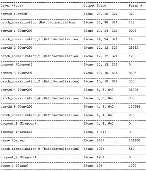
The CNN ensembles are built up with very accurate convolutional neural networks [3]. A Keras summary of such a CNN can be seen in the appendix. We used this CNN with structure in Table 8 as the background network of the label noise cleansing frameworks, too.

3.1. Comparison of the two cleansing frameworks

In order to get a better result we increased our dataset with 60 000 augmented images, where the augmentation was a little amount of random shift and rotation.

In our experiments the first step was to train a base-model with the cross entropy loss function with a high learning rate (lr = 1). After 20 epochs we saved our model and used it for both frameworks as a base-model. As a second step, we continued with the label changing phase of the two methods. Table 1 shows the parameters we used and how they worked on the different frameworks in this stage.

In the last two columns, we show how many labels were detected as incorrect on the whole dataset and in parentheses we show only the detected labels from the original dataset. The last column corresponds to an ensemble of a PENCIL and a Tanaka network, which was made by taking the average of the softmax outputs.

We also wanted to examine how differently the detection works in the case of these two frameworks. Table 2 contains the number of images, which were classified into the same new class according to the pairwise intersections of Tanaka, PENCIL and the ensemble of them. The table shows that different methods detect mostly the same label noise. Figure 2 shows some seemingly mislabeled training images,

(8)

which were found by both frameworks. The subcaptions contain the new labels and the highest scores generated by the cleansing methods. The Tanaka process seems to be more confident than PENCIL according to the higher peak scores. It can be generally concluded on the whole set of detected instances.

Table 1. Noisy label detection of ensembles on the training set with120 000samples.

Framework 𝛼 𝛽 lr 𝜆 epochs Detected labels Ensemble

PENCIL 0.05 0.6 0.1 600 30 71 (28) 75 (36)

Tanaka 1.1 0.6 0.05 - 20 116 (59)

Table 2. The number of identically detected images.

PENCIL Tanaka

Tanaka 54 (24) -

Ensemble 55 (24) 74 (36)

Original label: 3 New label: 5 Tanaka: 0.899 PENCIL: 0.641

Original label: 5 New label: 6 Tanaka: 0.887 PENCIL: 0.598 Figure 2. Some detected images with new labels and the

corresponding scores of Tanaka and PENCIL.

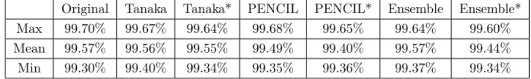
Then in this experiment we wanted to investigate how the exclusion of the detected labeled inputs affects the goodness of the CNN. Here we use a single very accurate CNN with structure in Table 8. In Table 3 we show that how the different training datasets performed with the same weight initialized models. The table contains the performance of our CNN model trained on the original augmented dataset and on its cleaned versions. Of course, they were evaluated on the test dataset. In Table 3, column ’Original’ contains the results of the CNN without cleaning the training set. Columns ’Tanaka’ and ’PENCIL’ contain the result of the CNN after cleaning with the Tanaka and PENCIL methods, respectively.

’Ensemble’ means that the cleaning was made by an ensemble of a Tanaka and a

(9)

PENCIL network, with weighting the same way as the previous case. The * symbol denotes the cases when we deleted the detected items only from the artificially created part of the training dataset. We repeated each experiment 30 times and in each case with a learning rate of 0.1 and a momentum of 0.2 for 30 epochs. In Table 3 we show the best, the worst and the mean of the 30 repetitions.

Table 3. Training with cleaned labels.

Original Tanaka Tanaka* PENCIL PENCIL* Ensemble Ensemble*

Max 99.70% 99.67% 99.64% 99.68% 99.65% 99.64% 99.60%

Mean 99.57% 99.56% 99.55% 99.49% 99.40% 99.57% 99.44%

Min 99.30% 99.40% 99.34% 99.35% 99.36% 99.37% 99.34%

We can see that the result depends on the cleaning method. We can also see that removing the misleading items makes the classification more stable in the following sense. The minimum is higher and the range is smaller after the use of each cleaning method than for the original raw dataset. For the original dataset the minimum is99.30% and the range is 99.70−99.40 = 0.40%while for Tanaka the minimum is 99.40% and the range is 0.27%. However, such simple cleaning techniques do not improve the average and the maximal performance.

3.2. Possibilities of improving a CNN ensemble classifier

Our final goal was to examine the opportunities of making an already accurate CNN ensemble classifier even better. An ensemble of 3 convolutional neural networks was trained before and after label noise cleansing. In our ensemble,3 CNNs with structure in Table 8 were used. For fair comparison, these networks were initialized with the same weights in each case. All of them were trained with a learning rate of0.1and a momentum of0.2 for30epochs.

The treating of the label noise was carried out in the following way: 3networks were trained with both frameworks. We took the average of the label estimations of the 6 networks and applied the NumPy argmax function. These were the new labels corresponding to the training examples.

In the following experiment the training data was slightly increased with24 000 augmented images, so the training set consisted of84 000examples in this setting.

For both noise cleansing frameworks, the training of the models began with 20 epochs using the cross entropy loss function and a momentum of0.3. In the second phase, the momentum was set to0.5 for the networks with Tanaka’s method and 0.1 for both of PENCIL’s optimizers, because of the nature of these techniques.

The other parameters can be seen in Table 4. Of course, the number of epochs in this table means the number of epochs in this phase. In the ’Detected labels’

column, there is the number of labels detected as noisy by the ensemble of the 3 networks corresponding to the methods. In parentheses, the number of noisy labels are shown in the original dataset. The last column contains the results of ensembling all the6networks.

(10)

Table 4. Noisy label detection of ensembles on the training set with84 000samples.

Framework 𝛼 𝛽 lr 𝜆 epochs Detected labels Ensemble

PENCIL 0.08 0.5 0.2 550 25 52 (27) 36 (24)

Tanaka 1.1 0.6 0.04 - 20 56 (32)

In the next part of the experiment, the different options of label noise handling are investigated. Table 5 contains the test performance of the CNN ensembles trained on this augmented dataset with the original labels, relabeling and deletion.

These results correspond to 20 runs in each case with the same 20×3weight set initialization. The first and third rows show the best and weakest performances, while the second line contains the mean of the 20 test accuracies.

Table 5. Performance of the CNN ensemble with different noise handling options.

CNN ensemble CNN ensemble CNN ensemble before after relabeling after deletion

Max 99.68% 99.71% 99.72%

Mean 99.663% 99.675% 99.673%

Min 99.58% 99.61% 99.60%

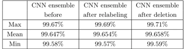
Finally, we wanted to investigate the opportunities of this CNN ensemble im- provement by using only the original60 000samples. In this setting, the parameters of the noise detecting ensemble are the same as before and this table corresponds to 3 PENCIL and 3 Tanaka networks, too. The number of labels detected as wrong are visible below and the performance of the CNN ensembles are shown in Table 7, in the same way as in Table 5.

Table 6. Noisy label detection of ensembles on the original MNIST dataset.

Framework Detected labels Ensemble

PENCIL 29 21

Tanaka 24

Table 7. Performance of the CNN ensemble with different noise handling options on the original MNIST.

CNN ensemble CNN ensemble CNN ensemble before after relabeling after deletion

Max 99.67% 99.69% 99.71%

Mean 99.647% 99.654% 99.658%

Min 99.58% 99.57% 99.59%

(11)

4. Conclusions

Machine learning methods developed for classification data with label noise can be applied to handle datasets containing some misleading items. These machine learning methods can be used for preprocessing the training data. After preprocessing any usual classification tool can be applied. Deleting some misleading items in the preprocessing phase is more promising than relabeling them. With preprocessing we can further improve the performance of very accurate convolutional networks, too. For preprocessing, ensembles of different noise correction methods (like the method of Tanaka et al. [8] and PENCIL of [10]) are promising. However, we have to be careful with relabeling and with removal of relabeled items, too. Relabeling means adding information to the training set artificially. If we relabel too many images, it may happen that we mislead the classifier with those modified labels.

The removal of the relabeled examples is also dangerous: it can cause information loss that degrades the performance of our models. (With high noise rates, it is obviously a wrong choice.) We can improve a classifier with those operations only if we find the right amount of training data to relabel or delete.

Acknowledgements. The authors are indebted to the referees for their valuable suggestions.

References

[1] G. Algan,I. Ulusoy: Image classification with deep learning in the presence of noisy labels: A survey, Knowledge-Based Systems 215 (2021), p. 106771,issn: 0950-7051, doi:https://doi.org/10.1016/j.knosys.2021.106771,

url:https://www.sciencedirect.com/science/article/pii/S0950705121000344.

[2] D. Arpit,S. Jastrzębski,N. Ballas,D. Krueger, E. Bengio,M. S. Kanwal,T.

Maharaj,A. Fischer,A. Courville,Y. Bengio,S. Lacoste-Julien:A Closer Look at Memorization in Deep Networks, in: ed. byD. Precup,Y. W. Teh, vol. 70, Proceedings of Machine Learning Research, International Convention Centre, Sydney, Australia: PMLR, Aug. 2017, pp. 233–242,

url:http://proceedings.mlr.press/v70/arpit17a.html.

[3] C. Deotte:How to choose CNN Architecture MNIST, 2018,

url:https://www.kaggle.com/cdeotte/how-to-choose-cnn-architecture-mnist.

[4] K. He,X. Zhang,S. Ren,J. Sun:Deep Residual Learning for Image Recognition, in: 2016 IEEE Conference on Computer Vision and Pattern Recognition (CVPR), 2016, pp. 770–778, doi:https://doi.org/10.1109/CVPR.2016.90.

[5] K. He, X. Zhang,S. Ren,J. Sun: Identity Mappings in Deep Residual Networks, in:

Computer Vision – ECCV 2016, ed. byB. Leibe,J. Matas,N. Sebe,M. Welling, Cham:

Springer International Publishing, 2016, pp. 630–645,isbn: 978-3-319-46493-0, doi:https://doi.org/10.1007/978-3-319-46493-0_38.

[6] Y. LeCun,C. Cortes,C. Burges:MNIST handwritten digit database, ATT Labs [Online].

Available: http://yann.lecun.com/exdb/mnist 2 (2010).

[7] T. Tajti:New voting functions for neural network algorithms, Annales Mathematicae et Informaticae 52 (2020), pp. 229–242,issn: 1787-6117,

doi:https://doi.org/10.33039/ami.2020.10.003.

(12)

[8] D. Tanaka,D. Ikami,T. Yamasaki,K. Aizawa:Joint Optimization Framework for Learn- ing With Noisy Labels, in: Proceedings of the IEEE Conference on Computer Vision and Pattern Recognition (CVPR), June 2018, pp. 5552–5560,

doi:https://doi.org/10.1109/CVPR.2018.00582.

[9] Tong Xiao,Tian Xia,Yi Yang,Chang Huang,Xiaogang Wang:Learning from massive noisy labeled data for image classification, in: 2015 IEEE Conference on Computer Vision and Pattern Recognition (CVPR), 2015, pp. 2691–2699,

doi:https://doi.org/10.1109/CVPR.2015.7298885.

[10] K. Yi,J. Wu:Probabilistic End-To-End Noise Correction for Learning With Noisy Labels, in: Proceedings of the IEEE/CVF Conference on Computer Vision and Pattern Recognition (CVPR), June 2019.

(13)

Appendix

Table 8. The Keras summary of the CNN that we used.

Model: "sequential"

_____________________________________________________________________________

Layer (type) Output Shape Param #

=============================================================================

conv2d (Conv2D) (None, 26, 26, 32) 320

_____________________________________________________________________________

batch_normalization (BatchNormalization) (None, 26, 26, 32) 128 _____________________________________________________________________________

conv2d_1 (Conv2D) (None, 24, 24, 32) 9248

_____________________________________________________________________________

batch_normalization_1 (BatchNormalization) (None, 24, 24, 32) 128 _____________________________________________________________________________

conv2d_2 (Conv2D) (None, 12, 12, 32) 25632

_____________________________________________________________________________

dropout (Dropout) (None, 12, 12, 32) 0

_____________________________________________________________________________

conv2d_3 (Conv2D) (None, 10, 10, 64) 8496

_____________________________________________________________________________

conv2d_4 (Conv2D) (None, 8, 8, 64) 36928

_____________________________________________________________________________

conv2d_5 (Conv2D) (None, 4, 4, 64) 102464

_____________________________________________________________________________

dropout_1 (Dropout) (None, 4, 4, 64) 0

_____________________________________________________________________________

flatten (Flatten) (None, 1024) 0

_____________________________________________________________________________

dense (Dense) (None, 128) 131200

_____________________________________________________________________________

batch_normalization_6 (BatchNormalization) (None, 128) 512 _____________________________________________________________________________

dropout_2 (Dropout) (None, 128) 0

_____________________________________________________________________________

dense_1 (Dense) (None, 10) 1290

=============================================================================

Total params: 327,242 Trainable params: 326,410 Non-trainable params: 832