Improvement in Satellite Image-Based Land Cover Classification with Landscape Metrics

(1)

remote sensing

Article

Improvement in Satellite Image-Based Land Cover Classification with Landscape Metrics

András Gudmann * , Nándor Csikós, Péter Szilassi and LászlóMucsi

Department of Physical Geography and Geoinformatics, University of Szeged, Egyetem utca 2, 6722 Szeged, Hungary; csikos@geo.u-szeged.hu (N.C.); toto@geo.u-szeged.hu (P.S.);

mucsi@geo.u-szeged.hu (L.M.)

* Correspondence: gudmandras@geo.u-szeged.hu

Received: 5 October 2020; Accepted: 28 October 2020; Published: 31 October 2020

Abstract:The use of an object-based image analysis (OBIA) method has recently become quite common for classifying high-resolution remote-sensed images. However, despite OBIA’s segmentation being equally useful for analysing medium-resolution images, it is not used for them as often. This study aims to analyse the effect of landscape metrics that have not yet been used in image classification to provide additional information for land cover mapping to improve the thematic accuracy of satellite image-based land cover mapping. To this end, multispectral satellite images taken by Landsat 8 Operational Land Imager (OLI) and Sentinel-2 Multispectral Instrument (MSI) during three different seasons in 2017 were analysed. The images were segmented, and based on these segments, four patch-level landscape metrics (mean patch size, total edge, mean shape index and fractal dimension) were calculated. A random forest classifier was applied for classification, and the Coordination of Information on the Environment Land Cover (CLC) 2018 database was used as reference data. According to the results, landscape metrics both with and without segmentation can significantly improve the overall accuracy of the classification over classification based on spectral values. The highest overall accuracy was achieved using all data (i.e., spectral values, segmentation, and metrics).

Keywords: land cover; land use; CORINE; landscape metrics; image classification; remote sensing;

random forest; Landsat 8; Sentinel-2

1. Introduction

The monitoring of land use and land cover (LULC) plays a vital role in the study of environmental change, management of natural resources (e.g., water and wastewater management and biomass monitoring) [1,2], urban planning, urban growth modelling [3,4] and creation of environmental policies for sustainable development [5–7]. Due to the expansion of artificial areas and an economic growth that is concomitant with increased human needs (which also causes extreme environmental stress), changes in LULC are steadily accelerating. Therefore, researchers need to maintain up-to-date, objective, and highly accurate and reliable LULC maps. Remote sensing is an essential tool for LULC classification because it provides reliable, extensive and high-temporal- and spatial-resolution data.

Currently, automated classification algorithms are the most common mapping method used on satellite imagery, as opposed to the visual interpretation of remotely sensed images. The greatest advantage of these methods is that they are suitable for extremely rapid land cover mapping of remote, uninhabited areas on a large (continental) scale; however, one drawback to their use is the uncertainty associated with their thematic accuracy. Classifications that are based solely on spectral values provide satisfying results, but there is always room for improvement in both the process and results. Improvements may

Remote Sens.2020,12, 3580; doi:10.3390/rs12213580 www.mdpi.com/journal/remotesensing

(2)

Remote Sens.2020,12, 3580 2 of 18

be found with attempts to combine applications of different sensor data, use multi-temporal satellite images or involvement of satellite image based indices in the classification [8,9].

Spectral indices are mainly used to improve the classification accuracy of land cover maps [10–13]

and few studies [14–20] have investigated the role played by landscape metrics in this field.

However, numerous studies have shown a relation between LULC and landscape, and thus, also between LULC and landscape metrics and their changes [15,21–23]. These papers have investigated not only the degree of relationship of certain LULC and landscape metrics, but have also investigated the effects of the scales and classifications on the landscape metrics themselves [24–26]. Landscape metric parameters are widely used as indicators of biodiversity, water quality and land cover change, and are still being further developed [27–30]. They offer a set of spatial tools for analysing entire landscapes and the arrangement and properties of their features. These metrics, which originated from the landscape ecology discipline, can provide information about the fragmentation of landscapes and the shapes of the patches. Furthermore, the landscape metrics, unlike segmentation, provide numeric values whereby certain categories can be generally described [31]. Because of these properties, landscape indices can provide additional information that improves LULC classification [32]. In this study, the effects of four landscape metrics (mean patch size, total edge, mean shape index, and fractal dimension) on the thematic accuracy of satellite image-based land cover classification are investigated.

Furthermore, the dependency of the landscape indices and segments on each other is analysed.

In addition, tests are conducted to determine which landscape metric is the most useful for land cover mapping. Based on statistical analysis, improvements in LULC classification are quantified and the scale sensitivity of the results is tested.

2. Study Areas

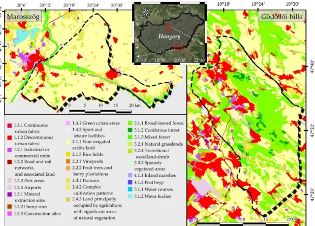
The study area contains two landscape units in Hungary with different physical geographical and land cover properties: Gödöll˝oi-hills and Marosszög (Figure1). The Gödöll˝oi-hills is a hilly region of Hungary comprising an area of 510 km². The region is between 138 and 344 m above sea level, sloping slightly to the southeast. This study area, which is located in central Hungary near Budapest, has a mosaic landscape with heterogeneous land cover characteristics. According to the Coordination of Information on the Environment (CORINE) Land Cover (CLC) 2018 database [33], the main land cover category here is the “non-irrigated arable land” (35.75% of the total area), but it also includes other significant land cover types, such as the ”broad-leaved forest” and “discontinuous urban fabric”

(29.64% and 10.39% of the total area, respectively) (Table1).

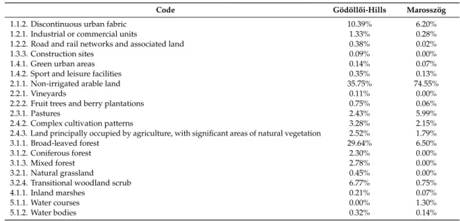
Table 1.Distribution of CLC classes in the two study areas.

Code Gödöll ˝oi-Hills Marosszög

1.1.2. Discontinuous urban fabric 10.39% 6.20%

1.2.1. Industrial or commercial units 1.33% 0.28%

1.2.2. Road and rail networks and associated land 0.38% 0.02%

1.3.3. Construction sites 0.09% 0.00%

1.4.1. Green urban areas 0.14% 0.07%

1.4.2. Sport and leisure facilities 0.35% 0.13%

2.1.1. Non-irrigated arable land 35.75% 74.55%

2.2.1. Vineyards 0.11% 0.00%

2.2.2. Fruit trees and berry plantations 0.75% 0.06%

2.3.1. Pastures 2.43% 5.99%

2.4.2. Complex cultivation patterns 3.28% 2.15%

2.4.3. Land principally occupied by agriculture, with significant areas of natural vegetation 2.52% 1.79%

3.1.1. Broad-leaved forest 29.64% 6.50%

3.1.2. Coniferous forest 2.30% 0.00%

3.1.3. Mixed forest 2.78% 0.00%

3.2.1. Natural grassland 0.45% 0.00%

3.2.4. Transitional woodland scrub 6.77% 0.75%

4.1.1. Inland marshes 0.21% 0.07%

5.1.1. Water courses 0.00% 1.30%

5.1.2. Water bodies 0.32% 0.14%

(3)

Remote Sens.2020,12, 3580 3 of 18

Remote Sens. 2020, 12, 3580 3 of 21

3.2.4. Transitional woodland scrub 6.77% 0.75%

4.1.1. Inland marshes 0.21% 0.07%

5.1.1. Water courses 0.00% 1.30%

5.1.2. Water bodies 0.32% 0.14%

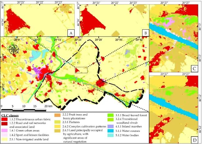
Figure 1. Land cover of the Marosszög and Gödöllői-hills study areas according to the CLC 2018 database.

Because of the proximity of the capital (Budapest), this study area is highly urbanised, with a relatively high proportion of the “discontinuous urban fabric” land cover type. Moreover, because of the highly variable elevation conditions of this hilly study area, the landscape pattern is more heterogeneous and mosaic than that in the other study area [34].

Due to the inclusion of several major classes and many patches, the mean land cover patch size of the total 349 CLC patches in the area is not very large (142 ha). The other study area, Marosszög, covers an area of 492 km² and is between 78 and 88 m above sea level. This alluvial plain, which is formed entirely by rivers, is relatively homogeneous and includes less diverse land cover characteristics, being covered mostly by agricultural land. Similar to the Gödöllői-hills, the majority of the land cover class here is also “non-irrigated arable land” (74.55% of the total area) (Table 1). Due to significant agricultural activity, the mean patch size is relatively high (352 ha) and the total number of land cover patches (polygons) is 166.

3. Materials and Methods 3.1. Remotely Sensed Data

For classification, three Landsat 8 and three Sentinel-2 satellite images were selected from three vegetation aspects (seasons) in 2017 (between March and October). The satellite data were processed with ERDAS Imagine 2020 and Sentinel Application Platform (SNAP)software. The satellite images obtained from the Landsat program were used for different classification purposes [35–37]. Landsat 8 is the newest satellite of its type. It scans the Earth’s surface in nine optical and two thermal bands

Figure 1. Land cover of the Marosszög and Gödöll˝oi-hills study areas according to the CLC 2018 database.

Because of the proximity of the capital (Budapest), this study area is highly urbanised, with a relatively high proportion of the “discontinuous urban fabric” land cover type. Moreover, because of the highly variable elevation conditions of this hilly study area, the landscape pattern is more heterogeneous and mosaic than that in the other study area [34].

Due to the inclusion of several major classes and many patches, the mean land cover patch size of the total 349 CLC patches in the area is not very large (142 ha). The other study area, Marosszög, covers an area of 492 km²and is between 78 and 88 m above sea level. This alluvial plain, which is formed entirely by rivers, is relatively homogeneous and includes less diverse land cover characteristics, being covered mostly by agricultural land. Similar to the Gödöll˝oi-hills, the majority of the land cover class here is also “non-irrigated arable land” (74.55% of the total area) (Table1). Due to significant agricultural activity, the mean patch size is relatively high (352 ha) and the total number of land cover patches (polygons) is 166.

3. Materials and Methods

3.1. Remotely Sensed Data

For classification, three Landsat 8 and three Sentinel-2 satellite images were selected from three vegetation aspects (seasons) in 2017 (between March and October). The satellite data were processed with ERDAS Imagine 2020 and Sentinel Application Platform (SNAP) software. The satellite images obtained from the Landsat program were used for different classification purposes [35–37]. Landsat 8 is the newest satellite of its type. It scans the Earth’s surface in nine optical and two thermal bands with different spatial resolutions (optical bands: 30 m; thermal bands: 100 m; panchromatic: 15 m).

Atmospheric-corrected Landsat images with surface reflectance values were ordered and downloaded from the Earth Resource Observation and Science (EROS) Processing Architecture (ESPA) system

(4)

Remote Sens.2020,12, 3580 4 of 18

(http://espa.cr.usgs.gov). The downloaded data’s thermal bands were then resampled to a 30-m spatial resolution, then all bands were resampled to 10 m spatial resolution. The base of the European Space Agency (ESA)’s Sentinel-2 program is a pair of optical satellites. Each satellite is mounted with a MultiSpectral Instrument, capable of capturing images in 13 optical bands; it was designed for use in other Earth observation satellites (e.g., Landsat and Spot). The visible-light and near-infrared bands have a spatial resolution of 10 m, while the other bands have spatial resolutions of either 20 or 60 m [38]. The Sentinel-2 images were resampled to 10 m resolution and corrected to the bottom-of-atmosphere reflectance.

3.2. Reference Land Cover Data (CORINE Land Cover 2018 Dataset)

The CLC program was launched by the European Community in 1985 with the aim of producing reliable land cover data for the member states of the Community, thus helping to develop a coherent environmental policy [39]. CLC databases are generated by visual interpretation. The advantage of this method is that the interpreter can consider several properties of the image (colour, tone, texture, size and shape) and use several additional sources of information (orthophotos, fieldwork, and site descriptions) to classify the areas in question. The disadvantage of this method, however, is that the quality of classification depends largely on the professional knowledge of the interpreter, and thus, the final result is highly subjective. Moreover, the process itself is time consuming due to the visual interpretation.

The land cover map of each member state is always prepared by the specialised organisation of the given member; the completed maps are then merged into a single database. To render the data usable and comparable, the maps are based on a uniform three-level classification system. Its smallest mapping unit is 25 ha, with a minimum width of 100 m for linear objects. The nomenclature of the classification system contains five classes at the first level, 15 at the second level and 44 at the third level [39]. The thematic accuracy of the CLC18 database is higher than 85% [33].

3.3. Calculation of Landscape Metrics

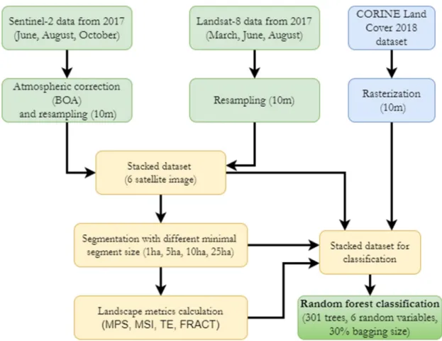
The processed sets of satellite images were stacked together and segmented with an edge detection method with different minimum segment sizes (1, 5, 10 and 25 ha) (Figure2). The segments contain only an ID number, but they are not pointing to one instance, and instead, indicate an instance group.

The main problem with these instance group IDs is that if an instance from a specific segment is not in the training set, the segment cannot improve the classification result (i.e., no rule is generated for that segment). Because of this, descriptors for the segment geometries are used. Based on the segments, four types of patch-level landscape metrics were calculated for each segment (polygon), which represented the size and shape characteristics of the segmented patches. The following landscape metrics were calculated by the V-Late 2 ArcGIS tool [40]: mean patch size (MPS), total edge (TE), mean shape index (MSI), and fractal dimension (MFRACT) (Table 2). The selection of the area- and shape-related landscape metrics was based on Szabó[41] and Walz [42]. These metrics are not completely redundant because they are not highly correlated with each other, which increases their usefulness in our classification [43,44]. MPS is an area-based landscape metric that describes the average landscape patch size and its distribution. TE is an edge-based landscape metric that shows the landscape patch type’s edge composition [21]. Both MPS and TE were used to represent the continuity of the landscape’s structure. To further describe changes in the geometrical complexity of a patch’s shape and the irregularity of its outer margin, the MSI and MFRACT were calculated [45]. MSI defines how compact the patches are on average (compared to a circle). MFRACT describes how complex or irregular the form of the landscape patch is; it comprises a normalised shape index in which the perimeter and area are log-transformed.

(5)

Remote Sens.2020,12, 3580 5 of 18

Remote Sens. 2020, 12, 3580 5 of 21

Figure 2. Pre-processing and classification processes.

Figure 2.Pre-processing and classification processes.

Table 2.Descriptions of the area, edge and shape metrics (based on [21,46]).

Feature Index Name and Description

Area MPS

Mean Patch Size MPS=

Pn j=1ai j

ni ,

wherea_ijrepresents the area of thej^thpatch in thei^thclass,n_irepresents the number of patches in thei^thclass andnrepresents the number of

patches (>0)

Edges TE

Total Edge TE=^P^m_k=1e_ik,

wheree_ikrepresents the edge length between thei^thandk^thpatch types andmrepresents the number of patch classes (≤0)

Shape Complexity

MSI

Mean Shape Index MSI=

Pn j=1

pij 2√

π∗aij

!

ni ,

wherep_ijrepresents the perimeter of thej^thpatch in classi^th,a_ij represents the area of thej^thpatch in classi^th,n_irepresents the number

of patches in thei^thclass andnrepresents the number of patches (≥1)

MFRACT

Mean Fractal Dimension MFRACT=

Pn j=1

2 lnpij lnaij

ni

wherep_ijrepresents the perimeter of thej^thpatch in classi^th,a_ij represents the area of thej^thpatch in classi^th,nirepresents the number of patches in thei^thclass andnrepresents the number of patches (1–2)

(6)

Remote Sens.2020,12, 3580 6 of 18

3.4. Classification

The classification of different land cover categories was performed on different data combinations, to evaluate the effects of the segmentation and landscape metrics. The landscape indices were used one-by-one and together, respectively, in the segment- and pixel-based classification methods (Figure2).

The third level of the CLC18 dataset was used as the reference data, which had good regional coverage and thematic accuracy, but its minimal mapping unit was relatively large (25 ha). Random points were generated (4000 points per class) as the training data. The training and test datasets were transformed to delimited text format, after which classification was performed using the WEKA software [47].

The random forest classification method was chosen, which is an assembly classifier designed with decision trees [48]. The random forest is a set of decision trees that, when combined, predict a majority voting scheme. The generalised error of the forest depends on two parameters: how accurate each individual classifier is and how independent the different classifiers are from each other (i.e., the strength of each tree in the forest and the correlation between them). While constructing the model, we can reduce the correlation between the trees by increasing the randomness, and thus, the generalised error as well [48]. The advantages here are the ability to classify large datasets with high accuracy and robustness vis-à-vis over-teaching. These properties make the random forest algorithm suitable for remote sensing applications [49]. A total of 301 trees and 6 random variables, with a 30% bagging size, was applied during the model’s formulation. To evaluate the performance of the random forest models, producer’s, user’s and overall accuracy, as well as different accuracy statistics (kappa, RMSE) of the classifiers, were examined.

4. Results

4.1. Influence of Segmentation on the Accuracy of Land Cover Mapping

According to the results, the application of the segmentation layer increased the overall accuracy by 1.15–4.21%, with the kappa coefficient varying between 0.64 and 0.76. Furthermore, a greater degree of improvement was achieved in the well-fragmented study area (Gödöll˝oi-hills), where the increase was between 3.98% and 4.21% (Table3). Regarding user accuracy, the greatest thematic accuracy increase was observed in mixed or complex land cover classes, such as “complex cultivation patterns”, “land principally occupied by agriculture, with significant areas of natural vegetation” and

“transitional woodland shrub” in both study areas (TablesA1andA3). In these class areas, the level of thematic accuracy increased by between 2.73% and 16.77%. Improvements in producer accuracy were observed in the same land cover classes as user accuracy, as well as some of the small-extent land cover categories, such as “road and rail networks and associated land” and “sport and leisure facilities”.

These land cover classes witnessed significant increases in accuracy (2.2–24.21%) (TablesA2andA4).

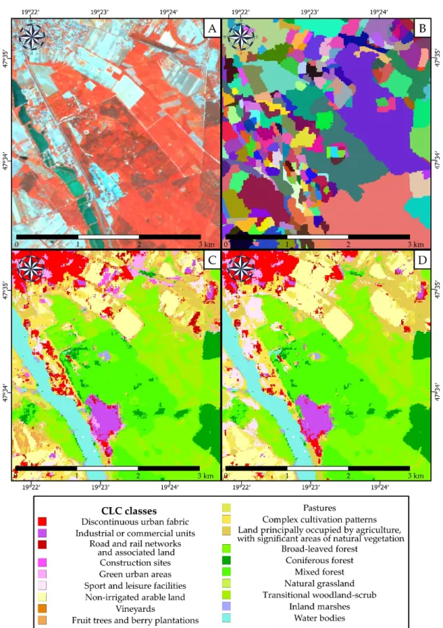
There were fewer incorrectly classified clusters and fewer inner scattered pixels in the clusters on the classified map. Thanks to these, more compacted land cover clusters were on the classified image (Figure3).

(7)

Remote Sens.2020,12, 3580 7 of 18

Remote Sens. 2020, 12, 3580 8 of 21

Figure 3. Effect of the segment layer on classification in the Gödöllői-hills study area: (A) original false colour satellite imagery, (B) segmented layer (5-ha minimal patch size), (C) classified map based on the spectral band, and (D) classified map based on spectral bands and the segments layer.

Figure 3.Effect of the segment layer on classification in the Gödöll˝oi-hills study area: (A) original false colour satellite imagery, (B) segmented layer (5-ha minimal patch size), (C) classified map based on the spectral band, and (D) classified map based on spectral bands and the segments layer.

(8)

Remote Sens.2020,12, 3580 8 of 18

Table 3.Overall accuracies and their increase under the influence of segmentation.

Study Area Data 1 ha +% 5 ha +% 10 ha +% 25 ha +%

Marosszög Spectral bands 87.02% - 86.92% - 87.02% - 87.02% -

Spectral bands+segments 88.50% 1.48% 88.46% 1.53% 90.16% 3.14% 88.17% 1.15%

Gödöll˝oi-hills

Spectral bands 66.81% - 66.86% - 66.81% - 66.81% -

Spectral bands+segments 70.91% 4.10% 71.07% 4.21% 70.79% 3.98% 70.92% 4.11%

4.2. Comparing the Accuracy of Land Cover Mapping Involving or Ignoring Landscape Indices

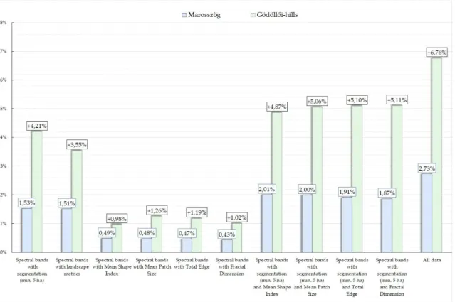
After determining the impact of segmentation on classification, the landscape metrics’ effects on LULC classification were analysed. For this analysis, the classification results of the metrics were selected, which were calculated on segments with a 5-ha minimum size. The overall accuracy improvement achieved without the segmentation layer was between 0.43% and 1.26%, and the combined use of all metrics led to a similar degree of improvement (1.51–3.55%). In addition, the use of segment layers, combined with one of the landscape metrics (MPS, MSI, TE or MFRACT), resulted in better thematic accuracy than a segment or metric layer alone. Moreover, the highest overall accuracy (89.65% with a kappa of 0.77 and 73.62% with a kappa of 0.67) was achieved for both study areas, using all the data (spectral values, segmentation and metrics) (Figure4).

Remote Sens. 2020, 12, 3580 9 of 21

Table 3. Overall accuracies and their increase under the influence of segmentation.

Study

Area Data 1 ha +% 5 ha +% 10 ha +% 25 ha +%

Marosszög

Spectral

bands 87.02% - 86.92% - 87.02% - 87.02% -

Spectral bands + segments

88.50% 1.48% 88.46% 1.53% 90.16% 3.14% 88.17% 1.15%

Gödöllői- hills

Spectral

bands 66.81% - 66.86% - 66.81% - 66.81% -

Spectral bands + segments

70.91% 4.10% 71.07% 4.21% 70.79% 3.98% 70.92% 4.11%

4.2. Comparing the Accuracy of Land Cover Mapping Involving or Ignoring Landscape Indices

After determining the impact of segmentation on classification, the landscape metrics’ effects on LULC classification were analysed. For this analysis, the classification results of the metrics were selected, which were calculated on segments with a 5-ha minimum size. The overall accuracy improvement achieved without the segmentation layer was between 0.43% and 1.26%, and the combined use of all metrics led to a similar degree of improvement (1.51–3.55%). In addition, the use of segment layers, combined with one of the landscape metrics (MPS, MSI, TE or MFRACT), resulted in better thematic accuracy than a segment or metric layer alone. Moreover, the highest overall accuracy (89.65% with a kappa of 0.77 and 73.62% with a kappa of 0.67) was achieved for both study areas, using all the data (spectral values, segmentation and metrics) (Figure 4).

Figure 4. Impact of data combinations on classification accuracy with 5-ha minimal segment size.

The user’s and producer’s accuracy values changed with greater magnitude (2–3 times) in the same land cover classes, just as in the case of segmentation (“complex cultivation patterns”, “land

Figure 4.Impact of data combinations on classification accuracy with 5-ha minimal segment size.

(9)

Remote Sens.2020,12, 3580 9 of 18

The user’s and producer’s accuracy values changed with greater magnitude (2–3 times) in the same land cover classes, just as in the case of segmentation (“complex cultivation patterns”, “land principally occupied by agriculture, with significant areas of natural vegetation” and “transitional woodland scrub”) and other small-extent classes (“construction sites”, “green urban areas”, “sport and leisure facilities”,

“vineyards” and “inland marshes”) (TablesA1–A4). According to these tables, the best metric in terms of accuracy improvement could not be determined but in some land cover classes the most effective metric could be selected (for example: in the Marosszög study area, based on the producer’s accuracy, at “Green urban areas” class, the MPS metric was the best). There were fewer internal scattered pixels in clusters, which created more compact segmented land cover patches (Figure5).

Remote Sens. 2020, 12, 3580 10 of 21

principally occupied by agriculture, with significant areas of natural vegetation” and “transitional woodland scrub”) and other small-extent classes (“construction sites”, “green urban areas”, “sport and leisure facilities”, “vineyards” and “inland marshes”) (Tables A1–A4). According to these tables, the best metric in terms of accuracy improvement could not be determined but in some land cover classes the most effective metric could be selected (for example: in the Marosszög study area, based on the producer’s accuracy, at “Green urban areas” class, the MPS metric was the best). There were fewer internal scattered pixels in clusters, which created more compact segmented land cover patches (Figure 5).

Figure 5. Differences between classification results based on only spectral bands and all data (including all landscape metric parameters) in the Marosszög study area. (A,C) classified maps based on spectral bands, and (B,D) classified maps based on all data.

4.3. Scale Dependency of Classification Accuracy

The influence of minimal segment size, and thus, the role played by scale were also investigated.

Three other minimal segment sizes were selected to analyse the sensitivity of the scales of 1 ha, which is the minimal mapping unit (MMU) of the Urban Atlas database; 25 ha, which is the MMU of the CLC database and has an intermediate size of 10 ha (Figure 6).

Figure 5.Differences between classification results based on only spectral bands and all data (including all landscape metric parameters) in the Marosszög study area. (A,C) classified maps based on spectral bands, and (B,D) classified maps based on all data.

4.3. Scale Dependency of Classification Accuracy

The influence of minimal segment size, and thus, the role played by scale were also investigated.

Three other minimal segment sizes were selected to analyse the sensitivity of the scales of 1 ha, which is the minimal mapping unit (MMU) of the Urban Atlas database; 25 ha, which is the MMU of the CLC database and has an intermediate size of 10 ha (Figure6).

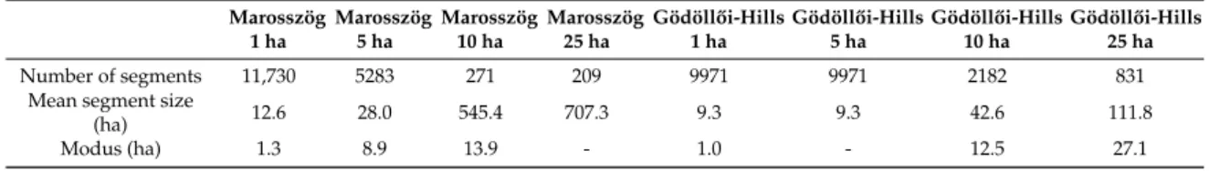
As a result of the different segmentations—in both study areas—the number of segments and the mean segment areas varied widely; the differences between the 1 and 25-ha minimal segment sizes were ~56% and ~12%, respectively (Table4).

(10)

Remote Sens.2020,12, 3580 10 of 18

Remote Sens. 2020, 12, 3580 11 of 21

Figure 6. Effect of different minimal segment sizes on segmentation in the Gödöllői-hills study area (red lines are polygons from the original CLC database). (A) segments with a 1-ha minimal patch size, (B) segments with a 5-ha minimal patch size, (C) segments with a 10-ha minimal patch size, and (D) segments with a 25-ha minimal patch size.

As a result of the different segmentations—in both study areas—the number of segments and the mean segment areas varied widely; the differences between the 1 and 25-ha minimal segment sizes were ~56% and ~12%, respectively (Table 4).

Figure 6.Effect of different minimal segment sizes on segmentation in the Gödöll˝oi-hills study area (red lines are polygons from the original CLC database). (A) segments with a 1-ha minimal patch size, (B) segments with a 5-ha minimal patch size, (C) segments with a 10-ha minimal patch size, and (D) segments with a 25-ha minimal patch size.

Table 4.Effect of using different minimum segment sizes.

Marosszög 1 ha

Gödöll ˝oi-Hills 1 ha

Number of segments 11,730 5283 271 209 9971 9971 2182 831

Mean segment size

(ha) 12.6 28.0 545.4 707.3 9.3 9.3 42.6 111.8

Modus (ha) 1.3 8.9 13.9 - 1.0 - 12.5 27.1

(11)

Remote Sens.2020,12, 3580 11 of 18

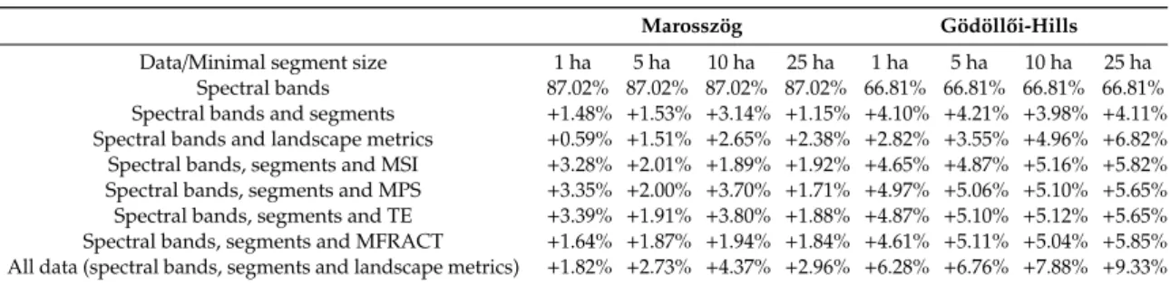
Contrary to the original assumption, the best overall accuracy values were achieved at less-fragmented areas with more segments (with 10-ha minimal segment sizes) and at well-fragmented areas with few segments (with 25-ha minimal segment sizes). In Marosszög, in six of the seven data variations, the best overall accuracy was achieved with the 10-ha minimal segment size; the data for other minimal segment sizes were better at only the “spectral bands, segments and MSI” (Table5).

Moreover, the data variation of “spectral bands and landscape metrics” resulted in only linear accuracy growth with increasing minimal segment size—the other scenarios’ values changed irregularly.

In contrast with Marosszög, the datasets obtained from the Gödöll˝oi-hills area exhibited the best overall accuracy values at the 25-ha minimal segment size (six of seven). In most cases, the increase was linearly dependent on the minimal segment size (Table5). Furthermore, in both study areas, the effect of the landscape metrics grew with the minimal segment size (both standalone and together), but the impact of the segmentation layer did not change remarkably.

Table 5.Overall accuracy increases with different datasets and minimal segment sizes.

Marosszög Gödöll ˝oi-Hills

Data/Minimal segment size 1 ha 5 ha 10 ha 25 ha 1 ha 5 ha 10 ha 25 ha Spectral bands 87.02% 87.02% 87.02% 87.02% 66.81% 66.81% 66.81% 66.81%

Spectral bands and segments +1.48% +1.53% +3.14% +1.15% +4.10% +4.21% +3.98% +4.11%

Spectral bands and landscape metrics +0.59% +1.51% +2.65% +2.38% +2.82% +3.55% +4.96% +6.82%

Spectral bands, segments and MSI +3.28% +2.01% +1.89% +1.92% +4.65% +4.87% +5.16% +5.82%

Spectral bands, segments and MPS +3.35% +2.00% +3.70% +1.71% +4.97% +5.06% +5.10% +5.65%

Spectral bands, segments and TE +3.39% +1.91% +3.80% +1.88% +4.87% +5.10% +5.12% +5.65%

Spectral bands, segments and MFRACT +1.64% +1.87% +1.94% +1.84% +4.61% +5.11% +5.04% +5.85%

All data (spectral bands, segments and landscape metrics) +1.82% +2.73% +4.37% +2.96% +6.28% +6.76% +7.88% +9.33%

5. Discussion

Previous research has proven the relation between LULC and landscape metrics [31], making such derivatives appropriate for increasing the classification efficiency. Using these metrics, the landscape characteristics of the LULC classes can be determined, thereby providing additional information to aid in classification. Prior studies have proven that some landscape metrics can increase the efficiency of LULC classification [14,16,18]. In contrast, the current study attempted to apply additional data to a more difficult classification task. A highly detailed reference database was used with more complex nomenclature, with 44 possible land cover classes and several basic landscape indicators (mean patch size, mean shape index, fractal dimension and total edge). Prior research showed the effectiveness of object-based (segment) image analysis of high-resolution images [50]. Segmentation forms the basis of object-based image analysis (OBIA) and is used to create homogeneous small objects from high-resolution satellite or aerial imagery [51]. Although this method has also been used on medium-resolution imagery, the goal has been the same: to examine an area of interest at greater scales and to obtain information about an image’s texture. Consistent with the results of previous research [14,52–55], the applicability of segmentation has been demonstrated in the land cover classification of medium-resolution satellite images. Although only pixel-based classification has been performed, segmentation could improve the accuracy of the classified images as compared to classification based on spectral values independent of the minimal segment size or the area’s fragmentation rate. In addition, the current study’s accuracy values indicate that the segmentation layer improves the classifier predictions for complex land cover classes, as well as the reliability of the classification of land cover maps’ small-extent categories.

A few researchers have studied the landscape indices derived from segments and their application’s effect on image classification [14,16,56]. Their results showed that basic segment information (e.g., area and perimeter) and complex metrics (e.g., shape complexity metrics) can improve classification accuracy. However, Chust et al. [56] found that the shape index and fractal dimension metrics yielded unconvincing results. In contrast to the aforementioned work, the current research rather effectively demonstrated the usefulness of applying landscape metrics such as mean patch size, mean shape index,

(12)

Remote Sens.2020,12, 3580 12 of 18

fractal dimension and total edge to LULC classification. According to the results, landscape metrics can improve the classification accuracy independent of segmentation and other landscape metrics, and the application of these landscape metrics with segmentation only improves the effects of the segmentation layer. The effects of the different landscape metrics changed depending on the scale. Thus, the best metric could not be determined, but the combined use of the metrics clearly yielded better results than those obtained by using them individually. Moreover, the highest degree of accuracy was achieved using all data (spectral bands, segments and landscape metric values). Consequently, segmentation and landscape metrics carry independent additional information about LULC, and both datasets can improve the classifier’s effectiveness. Moreover, the effects of additional data were most potent in the well-fragmented study area, where the landscape was mosaic and heterogeneous; however, there was a clear significant increase in accuracy in the other area as well.

Many researchers were interested in selecting the right scale for the segmentation and the determination of the minimal patch that would give the most suitable predictions [50]. Moreover, there is an example of the combined use of different scales [18]. In this study, four different scales were tested for LULC classification. Consistent with previously obtained results, the ideal segmentation scale could not be determined. The effect of the segmentation layer did not change meaningfully because of the different minimal segment size, but the landscape metrics’ effects clearly increased with the larger minimal segment size. Furthermore, in less-fragmented areas, better accuracy values were obtained with more segments, and in well-fragmented study areas, with fewer segments.

6. Conclusions

The usefulness of landscape metrics for LULC classification is a less-studied facet of remote sensing and image classification. However, the descriptors of a landscape and its structures and patterns provide information that is relevant to LULC. Our investigation proved the effective use of various shape- and size-related landscape metrics (mean patch size, total edge, mean shape index and fractal dimension) as input layers in the classification.

According to this study’s findings, the aforementioned indices could increase the prediction accuracy. Moreover, these landscape metrics improved the classification process even without the segmentation layer upon which the calculations were based. Moreover, differences in minimal segment size were found to increase the classification accuracy in different fragmented areas to differing degrees.

In both study areas, it was observed that the effect of the landscape metrics on classification accuracy was increased along with the minimal segment size. The best overall accuracies (Marosszög: 91.39% with a kappa of 0.81; Gödöll˝oi-hills: 76.14% with a kappa of 0.7) were obtained using all data (spectral bands, segmentation layer and all landscape metrics) with the 10-ha (Marosszög) and 25-ha (Gödöll˝oi-hills) minimal segment sizes. These results revealed that more research needs to be conducted on this topic;

using other reference data (LUCAS points, reference points from high-resolution satellite imagery or field survey data), we can examine the impact of a reference’s MMU, and the importance of the reference data’s reliability; with the separate use of the Landsat and Sentinel imagery, we can determine which data source is better for our methodology. Moreover, a future step is to combine the use of different scales and to apply other more sophisticated metrics that describe the landscape structure.

Author Contributions: Formal analysis A.G. and N.C.; Funding acquisition L.M.; Investigation A.G.;

Methodology A.G. and N.C.; Project administration A.G.; Supervision P.S. and L.M.; Writing—original draft A.G.; Writing—review & editing N.C., P.S. and L.M. All authors have read and agreed to the published version of the manuscript.

Funding:This research was supported by National Scientific Research Funds (Hungary) in support of the ongoing research, ‘Time series analysis of land cover dynamics using medium- and high-resolution satellite images’

(NKFIH 124648K), at the Department of Physical Geography and Geoinformatics of the University of Szeged.

Conflicts of Interest:The authors declare no conflict of interest.

(13)

Remote Sens.2020,12, 3580 13 of 18

Appendix A

Table A1.User’s accuracy values for different data combinations in the Marosszög study area, with 5 ha minimal segment size.

User’s Accuracy Spectral Bands

Spectral Bands and Segments

Spectral Bands and Landcsape

Metrics

Spectral Bands, Segments and

MSI

MPS

TE

FRACT

All Data

Discontinuous urban fabric 87.7% 89.5% 89.7% 90.3% 90.2% 90.0% 90.2% 91.5%

Road and rail networks and associated land 99.9% 99.9% 99.9% 99.9% 99.9% 99.9% 99.9% 99.9%

Green urban areas 99.9% 99.9% 99.9% 99.9% 99.9% 99.9% 99.9% 99.9%

Sport and leisure facilities 100.0% 100.0% 100.0% 100.0% 100.0% 100.0% 100.0% 100.0%

Non-irrigated arable land 87.4% 88.6% 88.3% 88.9% 88.9% 88.9% 88.7% 89.4%

Fruit trees and berry plantations 100.0% 100.0% 100.0% 100.0% 100.0% 99.9% 100.0% 100.0%

Pastures 86.3% 88.0% 88.1% 88.6% 88.4% 88.3% 88.5% 89.5%

Complex cultivation patterns 80.2% 84.3% 85.6% 85.5% 85.3% 85.4% 85.7% 87.9%

Land principally occupied by agriculture,

with significant areas of natural vegetation 77.7% 85.4% 85.9% 87.1% 87.0% 86.5% 87.0% 89.4%

Broad-leaved forest 83.4% 86.1% 87.8% 87.1% 87.1% 86.9% 87.3% 88.9%

Transitional woodland-scrub 83.5% 88.1% 88.9% 89.6% 89.9% 89.3% 89.5% 91.1%

Inland marshes 99.9% 99.9% 99.9% 99.9% 99.9% 99.9% 99.9% 99.9%

Water courses 97.4% 97.7% 97.7% 97.7% 97.8% 97.8% 97.7% 97.9%

Water bodies 100.0% 99.9% 100.0% 100.0% 100.0% 100.0% 100.0% 100.0%

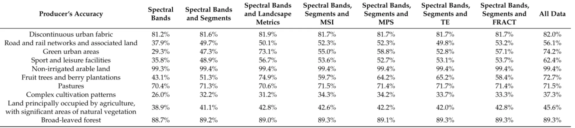
Table A2.Producer’s accuracy values for different data combinations in the Marosszög study area, with 5 ha minimal segment size.

Producer’s Accuracy Spectral Bands

Metrics

MSI

MPS

TE

FRACT

All Data

Pastures 70.4% 71.3% 70.6% 71.5% 71.4% 71.7% 71.4% 71.5%

(14)

Remote Sens.2020,12, 3580 14 of 18

Table A2.Cont.

Metrics

MSI

MPS

TE

FRACT

All Data

Inland marshes 51.0% 49.9% 63.7% 53.8% 52.0% 51.6% 55.9% 61.9%

Water courses 83.9% 84.4% 84.4% 84.8% 84.6% 84.3% 84.8% 85.0%

Water bodies 39.1% 45.3% 42.4% 44.9% 46.0% 46.1% 44.8% 45.9%

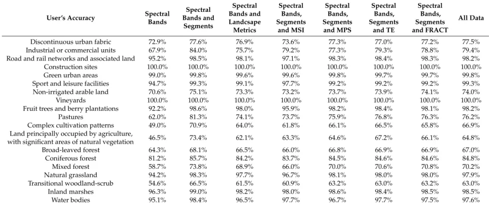
Table A3.User’s accuracy values for different data combinations in the Gödöll˝oi-hills study area, with 5 ha minimal segment size.

User’s Accuracy Spectral Bands

Spectral Bands and

Segments

Spectral Bands and Landcsape Metrics

Spectral Bands, Segments

and MSI

Spectral Bands, Segments and MPS

and TE

Spectral Bands, Segments and FRACT

All Data

Industrial or commercial units 67.9% 84.0% 75.7% 79.2% 77.3% 79.3% 78.8% 79.4%

Construction sites 100.0% 100.0% 100.0% 100.0% 100.0% 100.0% 100.0% 100.0%

Vineyards 100.0% 100.0% 100.0% 100.0% 100.0% 100.0% 100.0% 100.0%

Pastures 62.0% 81.3% 74.1% 73.7% 75.9% 76.8% 76.3% 76.2%

Coniferous forest 81.2% 85.7% 84.2% 83.7% 84.5% 84.6% 84.6% 84.8%

Mixed forest 58.7% 73.8% 68.9% 66.0% 70.0% 70.6% 70.8% 70.2%

Natural grassland 94.2% 98.3% 97.7% 96.7% 98.1% 98.0% 98.0% 97.9%

Inland marshes 96.3% 99.0% 98.2% 98.0% 98.6% 98.4% 98.5% 98.5%

Water bodies 95.1% 98.4% 96.5% 97.7% 96.7% 97.7% 97.5% 97.6%

(15)

Remote Sens.2020,12, 3580 15 of 18

Table A4.Producer’s accuracy values for different data combinations in Gödöll˝oi-hills study area, with 5 ha minimal segment size.

Spectral Bands and

Segments

Spectral Bands and Landcsape Metrics

and MSI

Spectral Bands, Segments and MPS

and TE

Spectral Bands, Segments and FRACT

All Data

Industrial or commercial units 45.8% 55.5% 40.8% 55.6% 53.4% 53.7% 56.0% 51.8%

Construction sites 10.8% 26.9% 20.7% 29.1% 28.8% 28.7% 28.7% 37.3%

Vineyards 30.7% 36.8% 55.8% 41.0% 41.0% 42.3% 43.3% 54.5%

Pastures 41.2% 42.0% 46.9% 43.1% 43.4% 44.0% 43.9% 47.2%

Coniferous forest 57.8% 60.6% 60.5% 61.2% 61.2% 61.4% 60.8% 62.3%

Mixed forest 44.8% 53.1% 48.4% 53.4% 53.2% 53.8% 54.3% 56.4%

Natural grassland 18.0% 23.4% 30.9% 26.0% 25.9% 25.9% 25.1% 31.8%

Inland marshes 15.8% 20.9% 25.0% 22.5% 23.7% 23.9% 23.6% 30.9%

Water bodies 43.6% 48.2% 43.9% 49.2% 49.1% 48.8% 50.2% 47.8%

(16)

Remote Sens.2020,12, 3580 16 of 18

References

1. Jensen, J.R.; Rutchey, K.; Koch, M.S.; Narumalani, S. Inland wetland change detection in the Everglades Water Conservation Area 2A using a time series of normalized remotely sensed data. Photogramm. Eng.

Remote Sens.1995,61, 199–209.

2. Gabiri, G.; Diekkrüger, B.; Näschen, K.; Leemhuis, C.; Van Der Linden, R.; Majaliwa, J.-G.M.; Obando, J.A.

Impact of Climate and Land Use/Land Cover Change on the Water Resources of a Tropical Inland Valley Catchment in Uganda, East Africa.Climate2020,8, 83. [CrossRef]

3. Jensen, J.R.; Cowen, D.J. Remote sensing of urban/suburban infrastructure and socio-economic attributes.

Photogramm. Eng. Remote Sens.1999,65, 611–622.

4. Mishra, B.K.; Mebeelo, K.; Chakraborty, S.; Kumar, P.; Gautam, A. Implications of urban expansion on land use and land cover: Towards sustainable development of Mega Manila, Philippines.Geojournal2019, 1–16. [CrossRef]

5. Nobre, C.A.; Sampaio, G.; Borma, L.S.; Castilla-Rubio, J.C.; Silva, J.S.; Cardoso, M. Land-use and climate change risks in the Amazon and the need of a novel sustainable development paradigm.Proc. Natl. Acad.

Sci. USA2016,113, 10759–10768. [CrossRef]

6. Shumilo, L.; Kolotii, A.; Lavreniuk, M.; Yailymov, B. Use of Land Cover Maps as Indicators for Achieving Sustainable Development Goals. In Proceedings of the IEEE International Geoscience and Remote Sensing Symposium, Valencia, Spain, 22–27 July 2018; pp. 830–833. [CrossRef]

7. Gibas, P.; Majorek, A. Analysis of Land-Use Change between 2012–2018 in Europe in Terms of Sustainable Development.Land2020,9, 46. [CrossRef]

8. Edash, J.; Mathur, A.; Foody, G.M.; Curran, P.J.; Chipman, J.W.; Lillesand, T.M. Land cover classification using multi-temporal MERIS vegetation indices.Int. J. Remote Sens.2007,28, 1137–1159. [CrossRef]

9. Zhou, T.; Li, Z.; Pan, J. Multi-Feature Classification of Multi-Sensor Satellite Imagery Based on Dual-Polarimetric Sentinel-1A, Landsat-8 OLI, and Hyperion Images for Urban Land-Cover Classification.

Sensors2018,18, 373. [CrossRef] [PubMed]

10. Fragoso-Campón, L.; Quirós, E.; Mora, J.; Gallego, J.A.G.; Durán-Barroso, P. Accuracy Enhancement for Land Cover Classification Using LiDAR and Multitemporal Sentinel 2 Images in a Forested Watershed.Proceedings 2018,2, 1280. [CrossRef]

11. Costachioiu, T.; Datcu, M. Land cover dynamics classification using multi-temporal spectral indices from satellite image time series. In Proceedings of the 2010 8th International Conference on Communications, Bucharest, Romania, 10–12 June 2010. [CrossRef]

12. Thakkar, A.K.; Desai, V.R.; Patel, A.; Potdar, M.B. Land Use/Land Cover Classification of Remote Sensing Data and Their Derived Products in a Heterogeneous Landscape of a Khan-Kali Watershed, Gujarat.

Asian J. Geoinform.2014,14, 1–12.

13. Ayala-Izurieta, J.E.; Márquez, C.O.; García, V.J.; Recalde, C.; Llerena, M.V.R.; Damián-Carrión, D.A.

Land Cover Classification in an Ecuadorian Mountain Geosystem Using a Random Forest Classifier, Spectral Vegetation Indices, and Ancillary Geographic Data.Geoscience2017,7, 34. [CrossRef]

14. Narumalani, S.; Zhou, Y.; Jelinski, D.E. Utilizing geometric attributes of spatial information to improve digital image classification.Remote Sens. Rev.1998,16, 233–253. [CrossRef]

15. Southworth, J.; Nagendra, H.; Tucker, C. Fragmentation of a Landscape: Incorporating landscape metrics into satellite analyses of land-cover change.Landsc. Res.2002,27, 253–269. [CrossRef]

16. Frohn, R.C. The use of landscape pattern metrics in remote sensing image classification.Int. J. Remote Sens.

2006,27, 2025–2032. [CrossRef]

17. Hurni, K.; Hett, C.; Epprech, M.; Messerli, P.; Heinimann, A. A Texture-Based Land Cover Classification for the Delineation of a Shifting Cultivation Landscape in the Lao PDR Using Landscape Metrics.Remote Sens.

2013,5, 3377–3396. [CrossRef]

18. Han, N.; Du, H.; Zhou, G.; Xu, X.; Ge, H.; Liu, L.; Gao, G.; Sun, S. Exploring the synergistic use of multi-scale image object metrics for land-use/land-cover mapping using an object-based approach.Int. J. Remote Sens.

2015,36, 3544–3562. [CrossRef]

19. Yu, L.; Su, J.; Li, C.; Wang, L.; Ze, L.; Yan, B. Improvement of Moderate Resolution Land Use and Land Cover Classification by Introducing Adjacent Region Features.Remote Sens.2018,10, 414. [CrossRef]

(17)

Remote Sens.2020,12, 3580 17 of 18

20. Grippa, T.; Georganos, S.; Zarougui, S.; Bognounou, P.; Diboulo, E.; Forget, Y.; Lennert, M.; VanHuysse, S.;

Mboga, N.; Wolff, E. Mapping Urban Land Use at Street Block Level Using OpenStreetMap, Remote Sensing Data, and Spatial Metrics.ISPRS Int. J. Geo-Inf.2018,7, 246. [CrossRef]

21. Uuemaa, E.; Antrop, M.; Roosaare, J.; Marja, R.; Mander, Ü. Landscape Metrics and Indices: An Overview of Their Use in Landscape Research.Living Rev. Landsc. Res.2009,3, 3. [CrossRef]

22. Fichera, C.R.; Modica, G.; Pollino, M. Land Cover classification and change-detection analysis using multi-temporal remote sensed imagery and landscape metrics.Eur. J. Remote Sens. 2012,45, 1–18. [CrossRef]

23. Szilassi, P.; Bata, T.; Szabó, S.; Czúcz, B.; Molnár, Z.; Mez˝osi, G. The link between landscape pattern and vegetation naturalness on a regional scale.Ecol. Indic.2017,81, 252–259. [CrossRef]

24. Lausch, A. Applicability of landscape metrics for the monitoring of landscape change: Issues of scale, resolution and interpretability.Ecol. Indic.2002,2, 3–15. [CrossRef]

25. Peng, J.; Wang, Y.; Ye, M.; Wu, J.; Zhang, Y. Effects of land-use categorization on landscape metrics: A case study in urban landscape of Shenzhen, China.Int. J. Remote Sens.2007,28, 4877–4895. [CrossRef]

26. Liu, D.; Hao, S.; Liu, X.; Li, B.; He, S.; Warrington, D.N. Effects of land use classification on landscape metrics based on remote sensing and GIS.Environ. Earth Sci.2012,68, 2229–2237. [CrossRef]

27. Singh, S.K.; Laari, P.B.; Mustak, S.; Srivastava, P.K.; Szabó, S. Modelling of land use land cover change using earth observation data-sets of Tons River Basin, Madhya Pradesh, India. Geocarto Int. 2017, 33, 1202–1222. [CrossRef]

28. Kumar, M.; Denis, D.M.; Singh, S.K.; Szabó, S.; Suryavanshi, S. Landscape metrics for assessment of land cover change and fragmentation of a heterogeneous watershed.Remote Sens. Appl. Soc. Environ.2018,10, 224–233. [CrossRef]

29. Csikos, N.; Szilassi, P. Impact of Energy Landscapes on the Abundance of Eurasian Skylark (Alauda arvensis), an Example from North Germany.Sustainability2020,12, 664. [CrossRef]

30. Szabó, S.; Csorba, P.; Szilassi, P. Tools for landscape ecological planning—Scale, and aggregation sensitivity of the contagion type landscape metric indices.Carpathian J. Earth Environ. Sci.2012,7, 127–136.

31. Jiao, L.; Liu, Y.; Li, H. Characterizing land-use classes in remote sensing imagery by shape metrics.ISPRS J.

Photogramm. Remote Sens.2012,72, 46–55. [CrossRef]

32. Sertel, E.; Topalo ˘glu, R.H.; ¸Sallı, B.; Algan, I.Y.; Aksu, G.A. Comparison of Landscape Metrics for Three Different Level Land Cover/Land Use Maps.ISPRS Int. J. Geo-Information2018,7, 408. [CrossRef]

33. Büttner, G.; Kosztra, B.CLC2018 Technical Guidelines, 2017, European Environmental Agency and European Topic Centre on Urban, Land and Soil Systems (ETC/ULS); Environment Agency: Vienna, Austria, 2017.

34. Szilassi, P. Land cover variability and the changes of land cover pattern in landscape units of Hungary.

J. Landsc. Ecol.2017,15, 131–138.

35. Mucsi, L.; Henits, L. Creating excess water inundation maps by sub-pixel classification of medium resolution satellite images.J. Environ. Geogr.2010,3, 31–40.

36. Phiri, D.; Morgenroth, J. Developments in Landsat Land Cover Classification Methods: A Review.Remote Sens.

2017,9, 967. [CrossRef]

37. Henits, L.; Mucsi, L.; Liska, C.M. Monitoring the changes in impervious surface ratio and urban heat island intensity between 1987 and 2011 in Szeged, Hungary.Environ. Monit. Assess.2017,189, 189. [CrossRef]

38. European Comission, Sentinel User Handbook and Exploration Tools (SUHET).Sentinel-2 User Handbook;

ESA: Paris, France, 2015; Issue 1, Revision 2.

39. Büttner, G.; Feranec, J.; Jaffrain, G.; Mari, L.; Maucha, G.; Soukup, T. The CORINE land cover 2000 project.

EARSeL eProc.2004,3, 331–346.

40. Comber, A.J.; Birnie, R.V.; Hodgson, M. Using landscape metrics to model land cover change. In Proceedings of the 9th Annual Conference of the International-Association-for-Landscape Ecology, Bangor, UK, 7–9 September 2000; pp. 143–161.

41. Szabó, S. Tájmetriai Mér˝oszámok Alkalmazási Lehet˝oségeinek Vizsgálata a Tájanalízisben. Ph.D. Thesis, University of Debrecen, Debrecen, Hungary, 2009.

42. Walz, U. Landscape Structure, Landscape Metrics and Biodiversity.Living Rev. Landsc. Res.2011,5, 5. [CrossRef]

43. Sinha, P.; Kumar, L.; Reid, N. Rank-Based Methods for Selection of Landscape Metrics for Land Cover Pattern Change Detection.Remote Sens. 2016,8, 107. [CrossRef]

44. Cushman, S.A.; McGarigal, K.; Neel, M.C. Parsimony in landscape metrics: Strength, universality, and consistency.

Ecol. Indic.2008,8, 691–703. [CrossRef]

(18)

Remote Sens.2020,12, 3580 18 of 18

45. Turner, M.G. Landscape Ecology: The Effect of Pattern on Process, 1. Annu. Rev. Ecol. Syst1989, 20, 171–197. [CrossRef]

46. Blaschke, T. The role of the spatial dimension within the framework of sustainable landscapes and natural capital.Landsc. Urban Plan.2006,75, 198–226. [CrossRef]

47. Eibe, F.; Mark, A.H.; Ian, H.W. The WEKA Workbench, Online Appendix. InData Mining: Practical Machine Learning Tools and Techniques, 4th ed.; Morgan Kaufmann: Cambridge, MA, USA, 2016.

48. Breiman, L. Random forests.Mach. Learn.2001,45, 5–32. [CrossRef]

49. Pal, M. Random forest classifier for remote sensing classification.Int. J. Remote Sens.2005,26, 217–222. [CrossRef]

50. Ma, L.; Li, M.; Ma, X.; Cheng, L.; Du, P.; Liu, Y. A review of supervised object-based land-cover image classification.ISPRS J. Photogramm. Remote Sens.2017,130, 277–293. [CrossRef]

51. Blaschke, T. Object based image analysis for remote sensing.ISPRS J. Photogramm. Remote Sens.2010,65, 2–16. [CrossRef]

52. Stuckens, J.; Coppin, P.; Bauer, M. Integrating Contextual Information with per-Pixel Classification for Improved Land Cover Classification.Remote Sens. Environ.2000,71, 282–296. [CrossRef]

53. Aguirre-Gutiérrez, J.; Seijmonsbergen, A.C.; Duivenvoorden, J.F. Optimizing land cover classification accuracy for change detection, a combined pixel-based and object-based approach in a mountainous area in Mexico.Appl. Geogr.2012,34, 29–37. [CrossRef]

54. Senthilnath, J.; Bajpai, S.; Omkar, S.; Diwakar, P.; Mani, V. An approach to multi-temporal MODIS image analysis using image classification and segmentation.Adv. Space Res.2012,50, 1274–1287. [CrossRef]

55. Zanotta, D.C.; Zortea, M.; Ferreira, M.P. A supervised approach for simultaneous segmentation and classification of remote sensing images.ISPRS J. Photogramm. Remote Sens.2018,142, 162–173. [CrossRef]

56. Chust, G.; Ducrot, D.; Pretus, J.L. Land cover mapping with patch-derived landscape indices.Landsc. Urban Plan.

2004,69, 437–449. [CrossRef]

Publisher’s Note:MDPI stays neutral with regard to jurisdictional claims in published maps and institutional affiliations.

©2020 by the authors. Licensee MDPI, Basel, Switzerland. This article is an open access article distributed under the terms and conditions of the Creative Commons Attribution (CC BY) license (http://creativecommons.org/licenses/by/4.0/).