remote sensing
Article
From Land Cover Map to Land Use Map: A Combined
Pixel-Based and Object-Based Approach Using Multi-Temporal Landsat Data, a Random Forest Classifier, and Decision Rules
Dang Hung Bui1,2,* and LászlóMucsi1
Citation: Bui, D.H.; Mucsi, L. From Land Cover Map to Land Use Map: A Combined Pixel-Based and Object- Based Approach Using Multi- Temporal Landsat Data, a Random Forest Classifier, and Decision Rules.
Remote Sens.2021,13, 1700. https://
doi.org/10.3390/rs13091700
Academic Editor: Jonathan C-W Chan
Received: 24 February 2021 Accepted: 25 April 2021 Published: 28 April 2021
Publisher’s Note:MDPI stays neutral with regard to jurisdictional claims in published maps and institutional affil- iations.
Copyright: © 2021 by the authors.
Licensee MDPI, Basel, Switzerland.
This article is an open access article distributed under the terms and conditions of the Creative Commons Attribution (CC BY) license (https://
creativecommons.org/licenses/by/
4.0/).
1 Department of Geoinformatics, Physical and Environmental Geography, University of Szeged, Egyetem utca 2, 6722 Szeged, Hungary; mucsi@geo.u-szeged.hu
2 Institute for Environmental Science, Engineering and Management, Industrial University of
Ho Chi Minh City, No. 12 Nguyen Van Bao Street, Go Vap District, Ho Chi Minh City 700000, Vietnam
* Correspondence: hungbui@geo.u-szeged.hu
Abstract: It is essential to produce land cover maps and land use maps separately for different purposes. This study was conducted to generate such maps in Binh Duong province, Vietnam, using a novel combination of pixel-based and object-based classification techniques and geographic information system (GIS) analysis on multi-temporal Landsat images. Firstly, the connection between land cover and land use was identified; thereafter, the land cover map and land use function regions were extracted with a random forest classifier. Finally, a land use map was generated by combining the land cover map and the land use function regions in a set of decision rules. The results showed that land cover and land use were linked by spectral, spatial, and temporal characteristics, and this helped effectively convert the land cover map into a land use map. The final land cover map attained an overall accuracy (OA) = 93.86%, with producer’s accuracy (PA) and user’s accuracy (UA) of its classes ranging from 73.91% to 100%. Meanwhile, the final land use map achieved OA = 93.45%, and the UA and PA ranged from 84% to 100%. The study demonstrated that it is possible to create high-accuracy maps based entirely on free multi-temporal satellite imagery that promote the reproducibility and proactivity of the research as well as cost-efficiency and time savings.
Keywords:land cover; land use; multi-temporal; pixel-based; object-based; segmentation; image classification; random forest; decision rules; Landsat-8
1. Introduction
Land cover is defined as “the observed (bio)physical cover on the earth’s surface” [1], including vegetation, water surface, bare rock, bare soil, buildings, and roads. Meanwhile, land use refers to “the arrangements, activities and inputs people undertake in a certain land cover type to produce, change or maintain it” [1]; in other words, land use is the way in which people use land cover types for one or more different purposes. Although they are defined differently and this issue has been discussed in previous studies [2–4], these two terms are still commonly used concurrently or interchangeably in many studies related to land cover and land use classification and mapping [5–7]. This problem may cause ambiguity or confusion for readers or map users [8], as well as certain difficulties in using such maps, because land use information is often used for planning [9] and making policy [10], while land cover information is often employed in environmental monitoring [11], modeling [12], and prediction [13].
Obviously, it is easier to observe and classify land cover types directly from aerial or satellite images than to do so with land use types [14]. However, there is a strong connection between land cover and land use [2,15], and once this relationship is clearly defined, land use types can be interpreted from land cover types. There have been attempts to use single or multiple remote sensing data independently [3,14,15] or in conjunction
Remote Sens.2021,13, 1700. https://doi.org/10.3390/rs13091700 https://www.mdpi.com/journal/remotesensing
Remote Sens.2021,13, 1700 2 of 24
with other ancillary data sources, such as census data [16], land use inventory data [17], social sensing data [18], and mobile-phone positioning data [19], to extract a land cover map and then translate it into a land use map, via a set of parameters and decision rules based on expert knowledge. Such studies have shown potential in producing a land use map from a land cover map based on remote sensing data. However, the reproducibility of their methods is a critical matter of concern. Most of these studies have used either commercial high-resolution satellite images and/or ancillary data, much of which was only available in their study regions. This matter may cause a limitation in repeating the methods of those studies in other study areas. With the availability of completely free remote sensing data sources (e.g., Landsat satellite family or Sentinel satellite family) that cover most of the terrestrial area of the Earth’s surface and are easy to access and download, it is necessary to have the research rely entirely on them to extract such maps. It not only enhances the reproducibility of the research methods but also their proactivity as well as cost-efficiency and time savings.
Vietnam is a developing country in Southeast Asia that has seen rapid urbaniza- tion and industrialization in recent years. According to the General Statistics Office of Vietnam [20], the population in Vietnam’s urban areas increased by an average of nearly 800,000 people each year in the 1999–2019 period. The rate of urbanization in the country, which was calculated as a percentage of the urban population per total population, reached 35.05% in 2019. The rate of urbanization is higher than the country average for megacities, such as Hanoi and Ho Chi Minh City, and also for provinces located in key economic zones, such as Binh Duong province. Specifically, in Binh Duong province, which is the area selected for this study, the rate of urbanization has increased rapidly since the 2000s up to now. In a period of ten years from 1995 to 2005, the urbanization rate only rose from 17.51% to 30.09%; however, in the following ten years (from 2005 to 2015), this rate grew rapidly from 30.09% to 76.72%. As of 2019, the rate reached 79.87%. As a result, in the process of urbanization and industrialization, the expansion of existing developed areas and the formation of new urban areas as well as new industrial and commercial regions have resulted in a rapid transformation of land use and land cover [21]. Therefore, it is necessary to use land cover and land use maps in near real time for planning and management activities.
In Vietnam, land use status maps are produced by the government at the local and national levels every five years. The basis for producing such maps consists of inventory data related to land changes, including land allocation, land lease, and change of land use purpose during the five-year inventory period [22]. The land use categories for the maps are up to five levels and 56 classes, which are very detailed and complex. The first version of this type of map was generated in 2005 (since the Act on Land 2003 was passed and implemented); thus, there is a lack of spatial data on land use for previous years. In addition, the five-year interval to produce the maps is not suitable for real-time management and research. Furthermore, the maps are extracted on computer-aided design (CAD) file formats, which make it difficult and time-consuming to convert and use them for geographic information system (GIS) analysis. Last but not least, it is difficult to access this data due to the government’s relatively complicated administrative system.
Meanwhile, a land cover map has not yet been produced by the government of Vietnam. Only a few studies have been done independently by researchers or organizations at the national [23,24] or local level [25–27]. However, depending on the purpose of each study, there are many dissimilarities in the land cover classification scheme as well as in the definitions of the classes in those schemes. In addition, a number of these studies also used the terms “land cover” and “land use” concurrently or interchangeably, which may cause a number of obstacles in using these maps, as noted. It should be highlighted that except for the SERVIR-Mekong [23] and Japan Aerospace Exploration Agency (JAXA) [24] programs for land use and land cover mapping for the whole of Vietnam, there are no other studies related to land cover classification in the selected study area.
Remote Sens.2021,13, 1700 3 of 24
With these issues in mind, this study was carried out in an effort to extract the land cover map and land use map of Binh Duong province separately. To achieve this objective, we proposed a novel combination of pixel-based and object-based classifications using random forest, decision rules, and free multi-temporal remote sensing data, specifically multi-temporal Landsat-8 imagery. The specific objectives of this study included:
• To identify the relationship between land cover and land use in Binh Duong province based on multi-temporal satellite images and field surveys.
• To test and assess the performance of the combination of pixel-based and object- based classification techniques and GIS analysis on multi-temporal Landsat images to generate a land cover map and a land use map separately.
2. Study Area
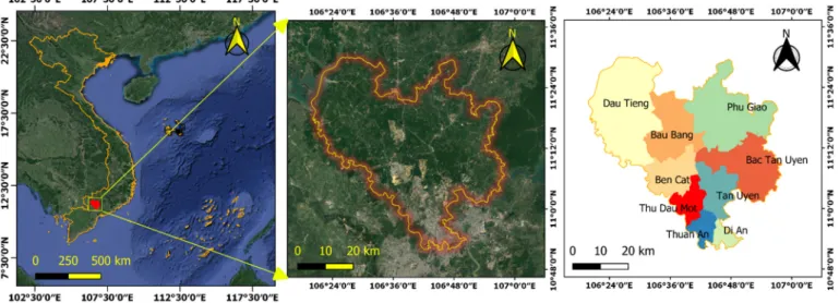
Binh Duong province is located in southeast Vietnam, between 10◦51046” and 11◦300 N latitude and between 106◦200and 106◦580E longitude (Figure1). The total area of the province is over 2694.64 km2, and its population is about 2.5 million people, of whom 79.87% live in urban areas as of 2019 [28].
Remote Sens. 2021, 13, x FOR PEER REVIEW 3 of 24
With these issues in mind, this study was carried out in an effort to extract the land cover map and land use map of Binh Duong province separately. To achieve this objective, we proposed a novel combination of pixel-based and object-based classifications using random forest, decision rules, and free multi-temporal remote sensing data, specifically multi-temporal Landsat-8 imagery. The specific objectives of this study included:
• To identify the relationship between land cover and land use in Binh Duong province based on multi-temporal satellite images and field surveys.
• To test and assess the performance of the combination of pixel-based and object- based classification techniques and GIS analysis on multi-temporal Landsat images to generate a land cover map and a land use map separately.
2. Study Area
Binh Duong province is located in southeast Vietnam, between 10°51′46″ and 11°30′
N latitude and between 106°20′ and 106°58′ E longitude (Figure 1). The total area of the province is over 2694.64 km2, and its population is about 2.5 million people, of whom 79.87% live in urban areas as of 2019 [28].
Figure 1. The study area.
Binh Duong’s climate is divided into two separate seasons, which are characterized by the tropical monsoon and sub-equatorial climates, with a rainy season from May to November, and a dry season from December to April of the following year. The total an- nual precipitation is about 2275 mm, in which the rainy season accounts for over 90%. The province has a stable geology, relatively flat terrain featuring ancient alluvial hills with an average height of 20–25 m and a slope of 3–15°. There are two large rivers (the Dong Nai and the Sai Gon) with many canals and other small streams.
3. Materials and Methods
The overall workflow is illustrated in Figure 2 and described in detail in the subsec- tions.
Figure 1.The study area.
Binh Duong’s climate is divided into two separate seasons, which are characterized by the tropical monsoon and sub-equatorial climates, with a rainy season from May to November, and a dry season from December to April of the following year. The total annual precipitation is about 2275 mm, in which the rainy season accounts for over 90%.
The province has a stable geology, relatively flat terrain featuring ancient alluvial hills with an average height of 20–25 m and a slope of 3–15◦. There are two large rivers (the Dong Nai and the Sai Gon) with many canals and other small streams.
3. Materials and Methods
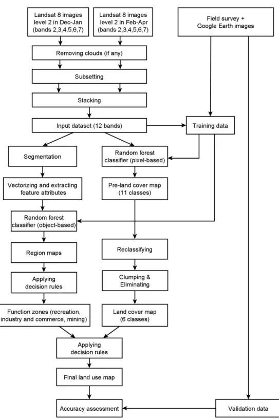
The overall workflow is illustrated in Figure2and described in detail in the subsections.
Remote Sens.2021,13, 1700 4 of 24
Remote Sens. 2021, 13, x FOR PEER REVIEW 4 of 24
Figure 2. The overall workflow.
3.1. The Main Land Cover and Land Use Classes in the Study Area
Based on the results of the field survey trip combined with observation of Landsat images and Google Earth history images, the main land cover types in Binh Duong prov- ince are defined below.
• Barren land: Totally bare soil areas without any cover or with very sparse vegetation or bare land areas partly covered with sunburned vegetation and/or very sparse fresh vegetation.
• Impervious surface with high albedo: Factories and commercial buildings whose ma- terial is often light-colored corrugated iron or concrete, or stone mining sites.
Figure 2.The overall workflow.
3.1. The Main Land Cover and Land Use Classes in the Study Area
Based on the results of the field survey trip combined with observation of Landsat images and Google Earth history images, the main land cover types in Binh Duong province are defined below.
• Barren land: Totally bare soil areas without any cover or with very sparse vegetation or bare land areas partly covered with sunburned vegetation and/or very sparse fresh vegetation.
Remote Sens.2021,13, 1700 5 of 24
• Impervious surface with high albedo: Factories and commercial buildings whose material is often light-colored corrugated iron or concrete, or stone mining sites.
• Impervious surface with low albedo: Residences, small commercial and office build- ings, roads whose material is often concrete, clay, corrugated iron, asphalt, or a mix of these materials, or stone mining sites.
• Grass: Fresh grass on cultivated grass farms, golf courses, and green spaces.
• Crops: Crops on farms and green spaces or plant nurseries with high density.
• Mature woody trees: Industrial trees, fruit trees, forests, and trees in green spaces which are of mature age with high coverage density.
• Young woody trees: Industrial trees, fruit trees, forests, and trees in green spaces which are young in age with low coverage density because their canopies/crowns are still separate.
• Water: Rivers, canals, lakes, ponds, and pools.
Meanwhile, determining the main land use classes in the study area was relatively difficult. Although the Vietnamese government has issued a current land use classifica- tion system [22], there were many land use categories with similar or very ambiguous definitions (e.g., defense land versus security land, land for religious facilities versus land for belief facilities, etc.), which caused difficulties in finding the relationship between land cover and land use. Additionally, many categories did not exist in the study area or occupied only a very small part and were thus unrepresentative of the study area.
Therefore, this study only used this land use classification system combined with the European Union’s Coordination of Information on the Environment (CORINE) land cover system [29] and the Food and Agriculture Organisation’s Land Cover Classification System (LCCS) [1] as references. The final land use categories were defined and modified based on the actual characteristics of the study area. Thus, land use classes in this study were defined as follows.
• Unused land: Areas where there are temporarily no construction works or which are leveled, or agricultural land in the harvest stage or in an early stage of the cultivation season with very young trees.
• Industry and commerce: Factories, buildings, a road network, and other built-up areas for production activities and/or commerce and services.
• Recreation and green space: Areas for relaxation and recreation activities, or areas for landscaping or creating a microclimate.
• Mixed residence: Houses, apartments, a road network, and other built-up areas for living and daily life activities. It may also include some entertainment buildings intermingled within residential areas.
• Mining sites: Areas for mining, exploitation, processing, and storing construction stone.
• Agriculture with annual plants: Agricultural land used for growing plants with the growth period from planting to harvesting not exceeding one year, such as rice, maize, vegetables, cultivated grass, etc., or plant nurseries.
• Agriculture with perennial plants: Agricultural land used for growing plants with the growth period from planting to harvesting over one year, such as fruit trees, industrial trees, and forests.
• Water surface: Water body surface.
3.2. Collecting and Pre-Processing Satellite Images
Landsat-8 Operational Land Imager (OLI) level 2 surface reflectance images for Binh Duong province (projection: WGS 84/UTM Zone 48N, path/row: 125/52) were ordered and downloaded from the United States Geological Survey (USGS) website [30]. The images (bands 2, 3, 4, 5, 6, 7) were collected at two consecutive periods:
• Period T1: from the end of November 2019 to the end of January 2020, corresponding to the period from the late rainy season to the early dry season.
Remote Sens.2021,13, 1700 6 of 24
• Period T2: from the beginning of February to the end of April 2020, corresponding to the period from the middle to the end of the dry season.
There were two reasons for selecting Landsat images at these two periods. Firstly, most of the study area was covered by dense clouds during the rainy season, i.e., from May to November; therefore, it was almost impossible to choose or to mosaic an image that was completely free of clouds in this period. Secondly, due to human activities, seasonal hydrological activities, and the characteristics of each land cover type, there was a transformation of land cover at some locations between the T1 and T2 periods. These changes might be used to improve the land cover classification and to interpret land use types. This will be discussed in detail in Section4.1.
As a result, at period T1, a completely cloud-free image acquired on 6 January 2020 was chosen. At period T2, images acquired on 23 February 2020 were selected. However, there was a small region in the study area covered by clouds on 23 February. Therefore, an image acquired on 7 February 2020, which was completely cloud-free in that small region, was additionally selected. Thus, the cloud region in the 23 February image was masked and replaced with the corresponding cloudless region in the 7 February image.
Then, selected images were subsetted to the study area and stacked together to create an input dataset with twelve bands (i.e., six bands in each period), which was ready for the next processing steps. The administrative boundary of the study area used for subsetting was downloaded from the Database of Global Administrative Areas (GADM) project website [31].
3.3. Collecting Training and Validation Data
A field survey trip to the study area was conducted from 18 January to 18 February 2020. From the results of the trip combined with the observations on the selected Landsat images at the T1 and T2 periods and the Google Earth History photos, a set of training and validation data was collected for classification and an accuracy assessment, respectively.
For the pixel-based classification, the two-stage sampling technique [32] was used. A total of 390 polygons were collected in homogeneous areas and assigned to the respective land cover classes. Subsequently, 70% of the polygons in each class were selected randomly, and all the pixels within them were extracted to create the training dataset (4909 pixels);
in the remaining number of polygons, 30% of the pixels were extracted periodically to create the validation data (586 pixels). It should be highlighted that because mining sites often had heterogeneous surfaces, consisting of interspersed high-albedo and low-albedo impervious surfaces, it was difficult to obtain a homogeneous region. Therefore, there were no polygons or points collected in these areas in this step.
For training in object-based classification, based on the segmented result, there were 399 and 349 segments selected for training in the first and second rounds, respectively. It should be noted that since an extended rectangular boundary was used in the segmentation step (see Section3.5), several segments that were outside the administrative boundary of the study area were selected to achieve the best result. Finally, to evaluate the accuracy of the final land use map, 586 points in the land cover validation dataset were used again, which were carefully assigned to the respective land use classes. In addition, 25 other points collected randomly at the mining sites were added. As a result, a total of 611 points were used at this stage.
The distribution of training and validation data depended on the proportion and spatial distribution of each class in the study area (Figure3). The detailed number of polygons and points for each class at each stage is summarized in AppendixA.
Remote Sens.Remote Sens. 2021, 13, x FOR PEER REVIEW 2021,13, 1700 7 of 247 of 24
Figure 3. The spatial distribution of training and validation data.
3.4. Pixel-Based Classification
The pixel-based approach was used in this study to produce the land cover map by applying random forest classifier and some post-classification techniques. The pixel-based approach was used due to its ability to generate a more detailed land cover map than one based on the object-based approach.
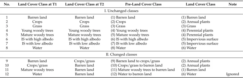
To pave the way for conversion from a land cover map to a land use map in the next steps, based on the fact that land cover at a location might be unchanged or changed from one type to another type between the two selected periods (see Section 4.1), an additional classification scheme with twelve classes was determined as in Table 1. It should be noted that despite the fact that there was a change from water to barren land at the coastal region of some water surfaces (e.g., reservoirs and lakes) between T1 and T2, that change only took place in a very small area. This issue made it difficult to obtain training and validation samples. Therefore, that type of change was ignored, and the classification process used only eleven classes.
Table 1. Pre-land cover and land cover classification scheme.
No. Land Cover Class at T1 Land Cover Class at T2 Pre-Land Cover Class Land Cover Class Note I. Unchanged classes
1 Barren land Barren land (1) Barren land (1) Barren land
2 Crops Crops (2) Crops (2) Annual plants
3 Grass Grass (3) Grass (3) Grass
4 Young woody trees Young woody trees (4) Young woody trees (4) Perennial plants 5 Mature woody trees Mature woody trees (5) Mature woody trees (4) Perennial plants 6 IS with high albedo IS with high albedo (6) IS with high albedo (5) Impervious surface 7 IS with low albedo IS with low albedo (7) IS with low albedo (5) Impervious surface
8 Water Water (8) Water (6) Water
II. Changed classes
9 Barren land Crops/grass (9) Barren land to crops/grass (2) Annual plants
10 Crops/grass Barren land (10) Crops/grass to barren land (2) Annual plants 11 Mature woody trees Barren land (11) Mature woody trees to barren land (1) Barren land
12 Water Barren land (12) Water to barren land (6) Water Ignored
Note: IS = Impervious surface.
Figure 3.The spatial distribution of training and validation data.
3.4. Pixel-Based Classification
The pixel-based approach was used in this study to produce the land cover map by applying random forest classifier and some post-classification techniques. The pixel-based approach was used due to its ability to generate a more detailed land cover map than one based on the object-based approach.
To pave the way for conversion from a land cover map to a land use map in the next steps, based on the fact that land cover at a location might be unchanged or changed from one type to another type between the two selected periods (see Section4.1), an additional classification scheme with twelve classes was determined as in Table1. It should be noted that despite the fact that there was a change from water to barren land at the coastal region of some water surfaces (e.g., reservoirs and lakes) between T1 and T2, that change only took place in a very small area. This issue made it difficult to obtain training and validation samples. Therefore, that type of change was ignored, and the classification process used only eleven classes.
Table 1.Pre-land cover and land cover classification scheme.
No. Land Cover Class at T1 Land Cover Class at T2 Pre-Land Cover Class Land Cover Class Note I. Unchanged classes
1 Barren land Barren land (1) Barren land (1) Barren land
2 Crops Crops (2) Crops (2) Annual plants
3 Grass Grass (3) Grass (3) Grass
4 Young woody trees Young woody trees (4) Young woody trees (4) Perennial plants 5 Mature woody trees Mature woody trees (5) Mature woody trees (4) Perennial plants 6 IS with high albedo IS with high albedo (6) IS with high albedo (5) Impervious surface 7 IS with low albedo IS with low albedo (7) IS with low albedo (5) Impervious surface
8 Water Water (8) Water (6) Water
II. Changed classes
9 Barren land Crops/grass (9) Barren land to crops/grass (2) Annual plants
10 Crops/grass Barren land (10) Crops/grass to barren land (2) Annual plants
11 Mature woody trees Barren land (11) Mature woody trees to barren land (1) Barren land
12 Water Barren land (12) Water to barren land (6) Water Ignored
Note: IS = Impervious surface.
Remote Sens.2021,13, 1700 8 of 24
A classified map (pre-land cover map) was produced using this classification scheme with the random forest algorithm [33], whose effectiveness in processing high-dimensional data has been proven to be fast and insensitive to overfitting [34]. The “randomForest”
package [35] was used on R software (version 3.6.3) for the classification procedure. In this process, the number of variables randomly sampled as candidates at each split (mtry) was set at the default value, which was equal to the square root of the total number of features.
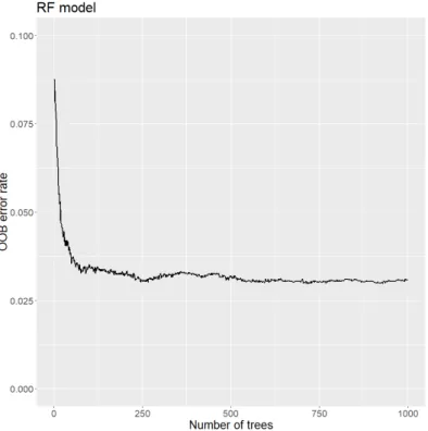
Meanwhile, the maximum number of trees (ntree) was decided based on the plot showing the relationship between ntree and the decrease of out-of-bag (OOB) error rates (Figure4).
As a result, ntree was set at 750 trees.
Remote Sens. 2021, 13, x FOR PEER REVIEW 8 of 24
A classified map (pre-land cover map) was produced using this classification scheme with the random forest algorithm [33], whose effectiveness in processing high-dimen- sional data has been proven to be fast and insensitive to overfitting [34]. The “random- Forest” package [35] was used on R software (version 3.6.3) for the classification proce- dure. In this process, the number of variables randomly sampled as candidates at each split (mtry) was set at the default value, which was equal to the square root of the total number of features. Meanwhile, the maximum number of trees (ntree) was decided based on the plot showing the relationship between ntree and the decrease of out-of-bag (OOB) error rates (Figure 4). As a result, ntree was set at 750 trees.
Figure 4. The relationship between out-of-bag (OOB) error rate and number of trees (ntree) in the random forest (RF) model for extracting the pre-land cover map.
Then, the pre-land cover map was re-classified from eleven to six classes to create the land cover map. The conversion of classes is also shown in Table 1. In addition, to remove
“salt and pepper” noise on the land cover map, the Clump and Eliminate functions in ERDAS IMAGINE 2020 software were used, respectively. Clumps (i.e., contiguous groups of pixels in one thematic class) smaller than four pixels were eliminated and given the value of nearby larger clumps. The final land cover map with the six classes was produced following this process.
In addition, a similar classification procedure was also performed on single images at T1 and T2 independently to compare the results with the classification output from the multi-temporal image.
3.5. Object-Based Classification
The purpose of this step was to produce land use function regions (i.e., industrial and commercial regions, mining regions, and recreation regions), which would be used to combine with the final land cover map to produce the final land use map. The object- based classification approach was used to create these regions. The object-based approach is capable of overcoming the spectral and spatial limitations of single pixels.
An extended rectangular boundary (Figure 3) was used at this stage instead of the administrative boundary to ensure landscape continuity in areas surrounding the admin- istrative boundary for more accurate segmentation. Firstly, the input raster dataset (12 Figure 4.The relationship between out-of-bag (OOB) error rate and number of trees (ntree) in the random forest (RF) model for extracting the pre-land cover map.
Then, the pre-land cover map was re-classified from eleven to six classes to create the land cover map. The conversion of classes is also shown in Table1. In addition, to remove
“salt and pepper” noise on the land cover map, the Clump and Eliminate functions in ERDAS IMAGINE 2020 software were used, respectively. Clumps (i.e., contiguous groups of pixels in one thematic class) smaller than four pixels were eliminated and given the value of nearby larger clumps. The final land cover map with the six classes was produced following this process.
In addition, a similar classification procedure was also performed on single images at T1 and T2 independently to compare the results with the classification output from the multi-temporal image.
3.5. Object-Based Classification
The purpose of this step was to produce land use function regions (i.e., industrial and commercial regions, mining regions, and recreation regions), which would be used to combine with the final land cover map to produce the final land use map. The object-based classification approach was used to create these regions. The object-based approach is capable of overcoming the spectral and spatial limitations of single pixels.
An extended rectangular boundary (Figure3) was used at this stage instead of the administrative boundary to ensure landscape continuity in areas surrounding the admin- istrative boundary for more accurate segmentation. Firstly, the input raster dataset (12
Remote Sens.2021,13, 1700 9 of 24
bands) was segmented using the Full Lambda Schedule (FLS) Image Segmentation func- tion in ERDAS software. In this study, after various experiments and visual analysis, the parameters were set as follows:
• Pixel:Segment Ratio: 50
• Relative Weights of Spectral: 0.5
• Relative Weights of Texture: 0.5
• Relative Weights of Size: 0.5
• Relative Weights of Shape: 0.5
• Size limits: minimum: 10; maximum: 1000
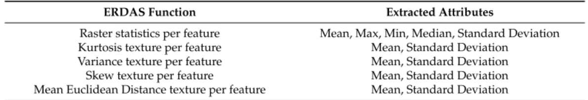
Subsequently, the segmentation image was converted to a polygon shapefile. From this shapefile and the input raster dataset, the following statistical and texture attributes of each raster band were extracted for each segment (i.e., each polygon) using a series of functions per feature in ERDAS (Table2). As a result, 156 attributes of each segment were extracted.
Table 2.Extracted attributes per feature.
ERDAS Function Extracted Attributes
Raster statistics per feature Mean, Max, Min, Median, Standard Deviation Kurtosis texture per feature Mean, Standard Deviation
Variance texture per feature Mean, Standard Deviation
Skew texture per feature Mean, Standard Deviation
Mean Euclidean Distance texture per feature Mean, Standard Deviation
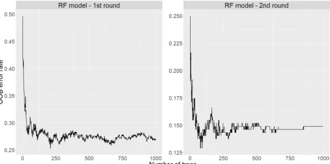
Finally, land use function regions were created using the random forest classifier on the extracted feature shapefile and then using spatial analysis techniques. The process is shown in Figure5. With the random forest algorithm, the ntree parameter was set to 650 trees for the first round and 600 trees for the second round (Figure6); meanwhile, the mtry parameter was also set to the default value. The spatial analysis was conducted in QGIS software (version 3.4.15) and the criteria were chosen based on a trial-and-error process.
There were two rounds of classification:
• The first round: to extract golf courses (recreation areas) and mining regions. The classification scheme included four potential classes: mining, recreation, industry and commerce, and other. The industrial and commercial region class was classified in this step in an effort to facilitate a better classification of the mining region.
• The second round: to extract industrial and commercial regions after subtracting recreation areas and mining areas in the first round. The classification scheme included two potential classes, industry and commerce, and other.
Remote Sens.2021,13, 1700 10 of 24
Remote Sens. 2021, 13, x FOR PEER REVIEW 10 of 24
Figure 5. Process for extracting land use function regions.
Figure 6. The relationship between OOB error rate and ntree in the RF models for extracting land use function regions.
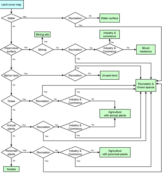
3.6. Producing the Land Use Map
The final land use map was created by combining the final land cover map and the land use function regions in a set of decision rules. The overall decision workflow is demonstrated in Figure 7.
Figure 5.Process for extracting land use function regions.
Remote Sens. 2021, 13, x FOR PEER REVIEW 10 of 24
Figure 5. Process for extracting land use function regions.
Figure 6. The relationship between OOB error rate and ntree in the RF models for extracting land use function regions.
3.6. Producing the Land Use Map
The final land use map was created by combining the final land cover map and the land use function regions in a set of decision rules. The overall decision workflow is demonstrated in Figure 7.
Figure 6.The relationship between OOB error rate and ntree in the RF models for extracting land use function regions.
3.6. Producing the Land Use Map
The final land use map was created by combining the final land cover map and the land use function regions in a set of decision rules. The overall decision workflow is demonstrated in Figure7.
Remote Sens.2021,13, 1700 11 of 24
Remote Sens. 2021, 13, x FOR PEER REVIEW 11 of 24
Figure 7. Decision rules for producing the land use map.
3.7. Accuracy Assessment
The accuracy of the land cover maps, function regions, and final land use map pro- duced at each processing step was assessed by both visual assessment and a confusion matrix with overall accuracy (OA), producer’s accuracy (PA), and user’s accuracy (UA) calculated. In addition, with the aim of assessing and comparing the accuracy of the gen- erated maps in more detail, this study also computed two other parameters, quantity dis- agreement (QD) and allocation disagreement (AD), instead of the Kappa coefficient, which has been proven by Pontius and Millones to be redundant or misleading [36]. Their study detailed the concept and method for calculating these two parameters.
Figure 7.Decision rules for producing the land use map.
3.7. Accuracy Assessment
The accuracy of the land cover maps, function regions, and final land use map pro- duced at each processing step was assessed by both visual assessment and a confusion matrix with overall accuracy (OA), producer’s accuracy (PA), and user’s accuracy (UA) calculated. In addition, with the aim of assessing and comparing the accuracy of the generated maps in more detail, this study also computed two other parameters, quantity disagreement (QD) and allocation disagreement (AD), instead of the Kappa coefficient, which has been proven by Pontius and Millones to be redundant or misleading [36]. Their study detailed the concept and method for calculating these two parameters.
Remote Sens.2021,13, 1700 12 of 24
4. Results
4.1. The Link between Land Cover and Land Use Types
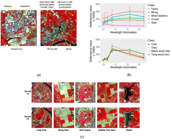
After defining the main land cover and main land use classes in the study area, the link between land cover and land use was interpreted by analyzing the spectral, spatial, and temporal characteristics of each land cover and land use type, as well as human and seasonal hydrological activities. The connection helped form a set of decision rules (see Section3.6) to efficiently convert the land cover map to a land use map. These connections are detailed below and illustrated in Figure8.
Remote Sens. 2021, 13, x FOR PEER REVIEW 12 of 24
4. Results
4.1. The Link between Land Cover and Land Use Types
After defining the main land cover and main land use classes in the study area, the link between land cover and land use was interpreted by analyzing the spectral, spatial, and temporal characteristics of each land cover and land use type, as well as human and seasonal hydrological activities. The connection helped form a set of decision rules (see Section 3.6) to efficiently convert the land cover map to a land use map. These connections are detailed below and illustrated in Figure 8.
(a) (b)
(c)
Figure 8. The characteristics of and connection between land cover and land use. (a) Spatial and visual characteristics; (b) Spectral characteristics; (c) Temporal characteristics.
• Barren land was often an area that was temporarily unused for any purpose. Its spec- tral signature overlapped partially with that of the impervious surfaces. However, the spectral signature of barren land regions fluctuated depending on the amount of vegetation scattered in the region. The less vegetation there was, the stronger the surface reflectance. Furthermore, the density and freshness of vegetation in barren land regions might slightly change with the seasons.
• Built-up areas and mining sites were all characterized by the domination of the im- pervious surface. The high density of the high-albedo impervious surface was usu- ally characteristic of the industrial and commercial regions. These areas often con- sisted of large, corrugated iron buildings (usually larger than 1000 m2/building) of a variety of colors, with each color marked by a different spectral signature. Thus, the Figure 8.The characteristics of and connection between land cover and land use. (a) Spatial and visual characteristics;
(b) Spectral characteristics; (c) Temporal characteristics.
• Barren land was often an area that was temporarily unused for any purpose. Its spectral signature overlapped partially with that of the impervious surfaces. However, the spectral signature of barren land regions fluctuated depending on the amount of vegetation scattered in the region. The less vegetation there was, the stronger the surface reflectance. Furthermore, the density and freshness of vegetation in barren land regions might slightly change with the seasons.
• Built-up areas and mining sites were all characterized by the domination of the impervious surface. The high density of the high-albedo impervious surface was usually characteristic of the industrial and commercial regions. These areas often consisted of large, corrugated iron buildings (usually larger than 1000 m2/building)
Remote Sens.2021,13, 1700 13 of 24
of a variety of colors, with each color marked by a different spectral signature. Thus, the spectral reflectance fluctuation in these regions was relatively wide in all bands.
Meanwhile, low-albedo impervious surface often fell within mixed residential areas, including private houses, blocks of flats, transportation networks, or small commercial buildings and office blocks with the building size often less than 500 m2. They were made up of different materials, such as corrugated iron, concrete, asphalt, brick, and clay tile. Hence, the value of each pixel in the Landsat image was a mixture of surface reflectance from these materials, and the spatial spectral variance was not too wide.
With stone-mining sites, they included impervious surface (both high and low albedo) and water, and the area of existing quarries was often larger than 20 ha. Furthermore, in general, in terms of temporal change, impervious surface was almost unchanged in a short time.
• Regions relevant to the domination of vegetation included recreation and green space regions and agricultural regions. Golf courses were dominated by a large fresh grass area. Meanwhile, green spaces could include woody or herbaceous plants with a small area and located in developed regions. For agricultural regions, in agricultural and forestry activities in Vietnam, woody trees were considered as perennial plants, and crops/cultivated grass were considered as annual plants. Comparing spectral signatures between grass, crops, and mature woody trees, it can be seen that although their curve shapes were relatively similar, fresh grass had the highest spectral re- flectance values in most bands, particularly in the NIR band. Mature woody tree regions seemed to have the lowest values in all bands. With young woody trees, because their canopies have not intersected yet, it led to low coverage density, and the spectral reflectance of such regions was a mixture of the plants and the ground.
This resulted in the spectral signature of this class being quite different from the other three vegetative classes. In addition, due to seasonal agricultural activities, cultivated grass/crops on farms might be changed to barren land and vice versa; meanwhile, grass on golf courses was unchanged.
• Mature woody tree regions could be changed to barren land after clear-cutting. This usually occurred on farms during the timber harvest (acacia, dipterocarps, etc.) or clear-cut poorly productive old trees for the new planting (with rubber, cashew, fruit trees, etc.). This also occurred in the area being leveled for construction activities in the future. The regions after such clear-cutting activities were considered as temporarily unused land.
• Water could be changed to barren land due to seasonal hydrological activities and vice versa. These semi-flooded areas were considered as falling within the water class.
4.2. Extracted Maps and Their Accuracy
4.2.1. The Pre-Land Cover Classification Result and the Final Land Cover Map
The OA, QD, and AD of the pre-land cover classification result achieved 89.76%, 5.68%, and 5.35%, respectively. The UA and PA of most classes achieved over 80%, in which the highest accuracy took place in the water class, which reached 100% for both PA and UA. In contrast, the crops class attained the poorest accuracy among eleven classes, with 53.33% of UA and 61.54% of PA. Many pixels of this class were misclassified in the mature woody tree class, whereas a number of pixels in the grass class were placed in this category. The misclassification from grass to crops also led to PA in the grass class also being low (65.22%).
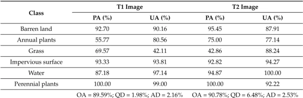
A final land cover map was generated from the result of the pre-land cover classifi- cation. For this map, except for the grass class, which attained PA = 73.91%, UA and PA achieved over 88% in all the other classes (Table3). Compared to the classification results from single images (Table4), the UA and PA of most classes of the final land cover map were equal to or higher than those of the single-date land cover maps, in which the most significant differences could be observed in the classes of grass and annual plants. The water class also experienced a slight increase in accuracy when using the multi-temporal
Remote Sens.2021,13, 1700 14 of 24
image. As a result, the OA of the classification result from multi-temporal images, which reached 93.86%, was higher than those of the single-date images, corresponding to OA = 89.59% for the land cover map at T1 and OA = 90.78% for the land cover map at T2. Simi- larly, the final land cover map also showed a lower disagreement in allocation compared to the land cover maps at T1 and T2, corresponding to AD of 1.51%, 2.16%, and 2.53%, respectively. The disagreement in terms of quantity for the final land cover map (QD = 4.59%) was also less than that of the land cover map at T2 (QD = 6.48%); however, it was higher than that at T1 (QD = 1.98%). However, in general, the total disagreements for all three maps were low and acceptable.
Table 3.Confusion matrix of final land cover map produced from the multi-temporal image.
Class Classification
Total PA (%)
BL AP GR IS WA PP
Referenced
BL 150 0 0 9 0 0 159 94.34
AP 5 77 0 0 0 5 87 88.51
GR 0 6 17 0 0 0 23 73.91
IS 11 0 0 184 0 0 195 94.36
WA 0 0 0 0 39 0 39 100.00
PP 0 0 0 0 0 83 83 100.00
Total 166 83 17 193 39 88 586
UA (%) 90.36 92.77 100.00 95.34 100.00 94.32
OA = 93.86%; QD = 4.59%; AD = 1.51%
Note: BL = barren land; AP = annual plants; GR = grass; IS = impervious surface; WA = water; PP = perennial plants; PA = producer’s accuracy; UA = user’s accuracy; OA = overall accuracy; QD = quantity disagreement;
AD = allocation disagreement.
Table 4.The accuracy of land cover maps produced from the single-date images.
Class T1 Image T2 Image
PA (%) UA (%) PA (%) UA (%)
Barren land 92.70 90.16 95.45 87.91
Annual plants 55.77 80.56 75.00 77.14
Grass 69.57 42.11 42.86 88.24
Impervious surface 93.33 93.81 92.82 94.27
Water 87.18 97.14 94.87 100.00
Perennial plants 100.00 99.00 100.00 92.22
OA = 89.59%; QD = 1.98%; AD = 2.16% OA = 90.78%; QD = 6.48%; AD = 2.53%
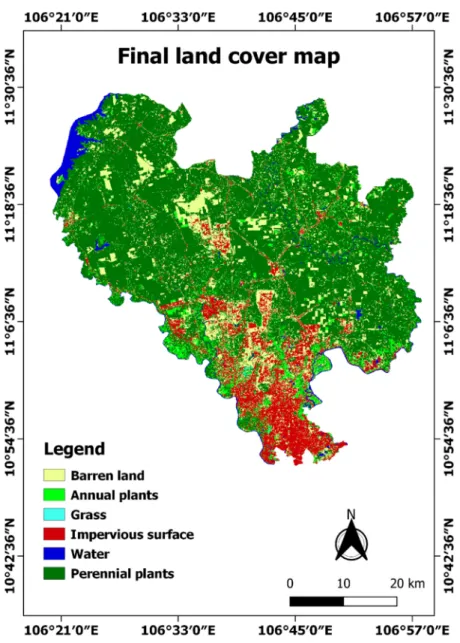
The final land cover map is illustrated in Figure9.
Remote Sens.2021,13, 1700 15 of 24
Remote Sens. 2021, 13, x FOR PEER REVIEW 15 of 24
Figure 9. Final land cover map.
4.2.2. Function Regions
Extracted function regions were assessed by visually comparing the study results with Landsat images and Google Earth History images. Some example regions are demon- strated in Figure 10. It can be seen that the shapes and sizes of the industrial parks, quar- ries, and golf courses compared relatively favorably to reality. Due to extracting from the remote sensing image, the boundaries of the image-based regions were not as smooth as they are in reality; however, in general, these image-based regions almost covered the entire land use areas. Although a few constructed buildings around quarries for pro- cessing and storing stone were classified under the mining function region, and some small, discrete stone storage yards were not included in this class, these miscategoriza- tions were acceptable to some extent. Overall, it was appropriate to use the generated function regions to produce the land use maps.
Figure 9.Final land cover map.
4.2.2. Function Regions
Extracted function regions were assessed by visually comparing the study results with Landsat images and Google Earth History images. Some example regions are demonstrated in Figure10. It can be seen that the shapes and sizes of the industrial parks, quarries, and golf courses compared relatively favorably to reality. Due to extracting from the remote sensing image, the boundaries of the image-based regions were not as smooth as they are in reality; however, in general, these image-based regions almost covered the entire land use areas. Although a few constructed buildings around quarries for processing and storing stone were classified under the mining function region, and some small, discrete stone storage yards were not included in this class, these miscategorizations were acceptable to some extent. Overall, it was appropriate to use the generated function regions to produce the land use maps.
Remote Sens.Remote Sens. 2021, 13, x FOR PEER REVIEW 2021,13, 1700 16 of 2416 of 24
Figure 10. Examples of extracted function regions.
4.2.3. Land Use Map
The final land use map is illustrated in Figure 11, and its accuracy assessment is demonstrated in Table 5. The map achieved 93.45% of OA, 4.58% of QD, and 1.52% of AD, as well as the UA and PA of its classes ranged from 84% to 100%. With visual evaluation, some pixels at the boundary areas of the mining sites were considered as a residence area.
This might come from the misclassification between barren land and impervious surface on the land cover map or generated mining function regions with inaccurate boundaries.
Table 5. Confusion matrix of the final land use map.
Class Classification
Total PA (%) UL IC RG MR MS AA AP WA
Referenced
UL 150 0 0 9 0 0 0 0 159 94.34
IC 3 79 0 0 0 0 0 0 82 96.34
RG 0 0 23 0 0 0 0 0 23 100.00
MR 8 6 0 99 0 0 0 0 113 87.61
MS 0 3 0 0 21 0 0 1 25 84.00
AA 5 0 0 0 0 77 5 0 87 88.51
AP 0 0 0 0 0 0 83 0 83 100.00
WA 0 0 0 0 0 0 0 39 39 100.00
Total 166 88 23 108 21 77 88 40 611
UA (%) 90.36 89.77 100.00 91.67 100.00 100.00 94.32 97.50 OA = 93.45%; QD = 4.58%, AD = 1.52%
Note: UN = unused land; IC = industry and commerce; RG = recreation and green space; MR = mixed residence; MS = mining site; AA = agriculture with annual plants; AP = agriculture with perennial plants; WA = water surface.
Figure 10.Examples of extracted function regions.
4.2.3. Land Use Map
The final land use map is illustrated in Figure11, and its accuracy assessment is demonstrated in Table5. The map achieved 93.45% of OA, 4.58% of QD, and 1.52% of AD, as well as the UA and PA of its classes ranged from 84% to 100%. With visual evaluation, some pixels at the boundary areas of the mining sites were considered as a residence area.
This might come from the misclassification between barren land and impervious surface on the land cover map or generated mining function regions with inaccurate boundaries.
Table 5.Confusion matrix of the final land use map.
Class Classification
Total PA (%)
UL IC RG MR MS AA AP WA
Referenced
UL 150 0 0 9 0 0 0 0 159 94.34
IC 3 79 0 0 0 0 0 0 82 96.34
RG 0 0 23 0 0 0 0 0 23 100.00
MR 8 6 0 99 0 0 0 0 113 87.61
MS 0 3 0 0 21 0 0 1 25 84.00
AA 5 0 0 0 0 77 5 0 87 88.51
AP 0 0 0 0 0 0 83 0 83 100.00
WA 0 0 0 0 0 0 0 39 39 100.00
Total 166 88 23 108 21 77 88 40 611
UA (%) 90.36 89.77 100.00 91.67 100.00 100.00 94.32 97.50
OA = 93.45%; QD = 4.58%, AD = 1.52%
Note: UN = unused land; IC = industry and commerce; RG = recreation and green space; MR = mixed residence; MS = mining site; AA = agriculture with annual plants; AP = agriculture with perennial plants; WA = water surface.
Remote Sens.2021,13, 1700 17 of 24
Remote Sens. 2021, 13, x FOR PEER REVIEW 17 of 24
Figure 11. Final land use map.
5. Discussion
The results of this study showed that land cover and land use in Binh Duong prov- ince were not only linked by spatial distribution and spectral properties but also by tem- poral characteristics. On the one hand, each land use type has its own spatial pattern and structure characterized by the properties of the land cover classes within it, such as com- position, spatial distribution, spectral signature, and dominant class as well as the shape and size of objects. On the other hand, the change or non-change of land cover at a given site over different times of the year may also demonstrate the manner in which humans interact with the land, thereby showing type of land use. In this study, characterizing the properties and finding the relationship between land cover and land use are considered as a vital key to producing a land cover map and a land use map from satellite images.
Once these relationships are clearly defined and the suitable classification schemes estab- lished, a set of decision rules can be established to demonstrate how to translate a land cover map into a land use map. Then, these maps can be efficiently extracted.
With our proposed procedure, the maps achieved high overall accuracy. It shows the potential of using a combination of pixel-based and object-based classification techniques and GIS techniques on free multi-temporal satellite images to effectively extract and trans- late a land cover map into a land use map. Many studies have also shown effectiveness in using a combination of these methods in the area of land cover and land use mapping [37–
Figure 11.Final land use map.
5. Discussion
The results of this study showed that land cover and land use in Binh Duong province were not only linked by spatial distribution and spectral properties but also by temporal characteristics. On the one hand, each land use type has its own spatial pattern and struc- ture characterized by the properties of the land cover classes within it, such as composition, spatial distribution, spectral signature, and dominant class as well as the shape and size of objects. On the other hand, the change or non-change of land cover at a given site over different times of the year may also demonstrate the manner in which humans interact with the land, thereby showing type of land use. In this study, characterizing the properties and finding the relationship between land cover and land use are considered as a vital key to producing a land cover map and a land use map from satellite images. Once these relationships are clearly defined and the suitable classification schemes established, a set of decision rules can be established to demonstrate how to translate a land cover map into a land use map. Then, these maps can be efficiently extracted.
With our proposed procedure, the maps achieved high overall accuracy. It shows the potential of using a combination of pixel-based and object-based classification tech- niques and GIS techniques on free multi-temporal satellite images to effectively extract and translate a land cover map into a land use map. Many studies have also shown effec- tiveness in using a combination of these methods in the area of land cover and land use
Remote Sens.2021,13, 1700 18 of 24
mapping [37–42]; however, the difference in this study is the production of a land cover map and land use map separately, which these previous studies have not done.
As the final land use map in our research was generated by combining the land cover map and the land use function regions in a set of decision rules, its accuracy depended on that of the combined components. The advantages to and limitations in how these components are produced are discussed in detail below.
First of all, the method for collecting training and validation data in our study is close to the stratified random sampling method. The distribution of the training and validation data depends on the spatial distribution and the proportion of each class in the study area. For example, in areas where many different types of land cover and land use classes are presented, e.g., in the southern part of the province, sampling density is higher than in other parts (Figure3). In addition, the number of samples of the dominant classes, such as the woody tree or impervious surface classes, is also greater than those of others (AppendixA). Thus, it can be assumed that there is no bias in the research results, thereby ensuring the accuracy and reliability of the generated maps. Furthermore, in the case of a large study area, where more samples need to be collected, it is more appropriate to use the stratified random sampling method, because it ensures that rare classes are not ignored, and it also requires a smaller sample size than the simple random sampling method. This can help save time and effort.
In land cover mapping, in our study, the higher the overall accuracy, the higher ac- curacy within classes and the low total disagreement of the final land cover map have shown a certain efficiency when using multi-temporal images in a pixel-based classifi- cation compared to using single-date images. These results are consistent with those of Feng et al. [43], Henits et al. [44], Yang et al. [45], and Zoungrana et al. [46]. The pixel- based classification results using a single-date satellite image often encounter common misclassification problems, such as those between impervious surface and barren land [47], between dark impervious surface, object-cast shadow, and water [48], between water boundary areas and barren land [49], between sparse vegetation and barren land [50], and between different vegetation classes [51], due to the spectral similarity between the classes.
However, using multi-date images can provide additional useful information to increase classification efficiency [46]. As noted in Section4.1, there may be a change in land cover and/or its features between two or more time points, which leads to a change in the spectral signature in some areas with no change in others. Therefore, the spectral similarities of these classes may be reduced or removed when using multi-temporal images; thus, it is possible to reduce misclassification. In addition to an improvement in land cover mapping, using multi-temporal images could also facilitate the extraction of land use information, paving the way for land use mapping. For example, by detecting the change/non-change between grass/crops and barren land, it was possible to distinguish agricultural areas from recreation areas and agricultural areas from unused land.
However, taking a more detailed look at the pre-land cover classification result, a high misclassification between some classes, especially between unchanged vegetation classes, still occurred in our research. This can be explained as follows: since only two temporal Landsat-8 images in the dry season are used in this study, they are not able to cover all situations of land cover change at different time points in a year. Meanwhile, depending on the characteristics of crop and farming techniques, the timing of cultivation and harvest on different parcels may not be the same; therefore, there are some parcels covered by crops at both of the selected periods. This problem, combined with the spectral similarity of crops, grass, and woody trees, led to a high misclassification from grass to crops and from crops to mature woody trees. It should be noted that in addition to reducing the accuracy of the land cover map, the misclassification can also affect the extraction of wrong land use information in the steps that follow. Therefore, this limitation should be considered in further studies to improve the accuracy of extracted maps. Adding more remote sensing image data at different times should be considered for the classification process. In addition, other optical image data such as Sentinel-2 may be used in combination to address the
Remote Sens.2021,13, 1700 19 of 24
problem of some cloud-covered areas in the dry season. In the rainy season, as noted, it is almost impossible to select or to mosaic an optical image that is completely free of clouds in the study area. Hence, it is suggested that a combination with synthetic aperture radar (SAR) images (e.g., Sentinel-1 imagery), which are unaffected by clouds [52], should be experimented with. We will pursue this in further studies.
It is a fact that a land use type consists of many land cover types, not only one [3].
Although industrial and commercial regions, for instance, are dominated by impervious surfaces with high albedo, they may also consist of impervious surfaces with low albedo, such as roads, yards, or small offices, or even grass and trees that are considered as landscaping. Similarly, mining site regions also comprise both high- and low-albedo impervious surfaces as well as water. Thus, if based only on a pixel-based classification—
i.e., based solely on spectral characteristics—it is difficult to form boundaries between regions with different land use types. In this study, the segmentation technique and object-based classification have shown the suitability of creating such boundaries and then forming land use function regions. Firstly, segmentation techniques group adjacent pixels into a homogeneous object (i.e., a segment) with clear boundaries by taking into account not only spectral properties but also spatial information, such as texture, shape, and size.
Then, the multiple statistical and texture variables are calculated from twelve bands of multi-temporal images based on the value distribution and spatial relationship of all the pixels within each segment; thus, they characterize the spatial distribution of land cover, in other words, the spatial pattern and structure of the land use type, within each segment.
This captured information is the basis for classifying segments into land use classes. A comparison of value distribution of some derived attributes between different land use types is illustrated in Figure12. Similar to pixel-based classification, adding more temporal images can help capture more spectral and spatial information, resulting in more efficient segmentation and classification. Despite a potential higher time cost in the processing, it is deemed acceptable.
Remote Sens. 2021, 13, x FOR PEER REVIEW 19 of 24
process. In addition, other optical image data such as Sentinel-2 may be used in combina- tion to address the problem of some cloud-covered areas in the dry season. In the rainy season, as noted, it is almost impossible to select or to mosaic an optical image that is completely free of clouds in the study area. Hence, it is suggested that a combination with synthetic aperture radar (SAR) images (e.g., Sentinel-1 imagery), which are unaffected by clouds [52], should be experimented with. We will pursue this in further studies.
It is a fact that a land use type consists of many land cover types, not only one [3].
Although industrial and commercial regions, for instance, are dominated by impervious surfaces with high albedo, they may also consist of impervious surfaces with low albedo, such as roads, yards, or small offices, or even grass and trees that are considered as land- scaping. Similarly, mining site regions also comprise both high- and low-albedo impervi- ous surfaces as well as water. Thus, if based only on a pixel-based classification—i.e., based solely on spectral characteristics—it is difficult to form boundaries between regions with different land use types. In this study, the segmentation technique and object-based classification have shown the suitability of creating such boundaries and then forming land use function regions. Firstly, segmentation techniques group adjacent pixels into a homogeneous object (i.e., a segment) with clear boundaries by taking into account not only spectral properties but also spatial information, such as texture, shape, and size.
Then, the multiple statistical and texture variables are calculated from twelve bands of multi-temporal images based on the value distribution and spatial relationship of all the pixels within each segment; thus, they characterize the spatial distribution of land cover, in other words, the spatial pattern and structure of the land use type, within each segment.
This captured information is the basis for classifying segments into land use classes. A comparison of value distribution of some derived attributes between different land use types is illustrated in Figure 12. Similar to pixel-based classification, adding more tem- poral images can help capture more spectral and spatial information, resulting in more efficient segmentation and classification. Despite a potential higher time cost in the pro- cessing, it is deemed acceptable.
Figure 12. Value distribution of some derived attributes of classes.
It should be highlighted that at the segmentation stage, the setting of parameters will affect the performance of segmentation [53]. The errors of over-segmentation and under- segmentation [54] may lead to incorrect boundaries. However, there are no perfect param- eters for this stage [55]. The performance of segmentation results is mostly based on user experience [53], and the setting also depends on satellite image resolutions and the spatial Figure 12.Value distribution of some derived attributes of classes.
It should be highlighted that at the segmentation stage, the setting of parameters will affect the performance of segmentation [53]. The errors of over-segmentation and under-segmentation [54] may lead to incorrect boundaries. However, there are no perfect parameters for this stage [55]. The performance of segmentation results is mostly based on user experience [53], and the setting also depends on satellite image resolutions and the