On the universality of the quantum approximate optimization algorithm

https://doi.org/10.1007/s11128-020-02748-9

On the universality of the quantum approximate optimization algorithm

M. E. S. Morales¹·J. D. Biamonte¹·Z. Zimborás^2,3,4

Received: 20 September 2019 / Accepted: 4 July 2020

© The Author(s) 2020

Abstract

The quantum approximate optimization algorithm (QAOA) is considered to be one of the most promising approaches towards using near-term quantum computers for practical application. In its original form, the algorithm applies two different Hamil- tonians, called the mixer and the cost Hamiltonian, in alternation with the goal being to approach the ground state of the cost Hamiltonian. Recently, it has been suggested that one might use such a set-up as a parametric quantum circuit with possibly some other goal than reaching ground states. From this perspective, a recent work (Lloyd, arXiv:1812.11075) argued that for one-dimensional local cost Hamiltonians, com- posed of nearest neighbour ZZ terms, this set-up is quantum computationally universal and provides a universal gate set, i.e. all unitaries can be reached up to arbitrary pre- cision. In the present paper, we complement this work by giving a complete proof and the precise conditions under which such a one-dimensional QAOA might produce a universal gate set. We further generalize this type of gate-set universality for cer- tain cost Hamiltonians with ZZ and ZZZ terms arranged according to the adjacency structure of certain graphs and hypergraphs.

B

zimboras.zoltan@wigner.mta.hu M. E. S. Morales

mauro990@gmail.com http://quantum.skoltech.ru J. D. Biamonte

j.biamonte@skoltech.ru http://quantum.skoltech.ru

1 Deep Quantum Laboratory, Skolkovo Institute of Science and Technology, 3 Nobel Street, Moscow, Russia 121205

2 Wigner Research Centre for Physics of the Hungarian Academy of Sciences, Budapest, Hungary 3 MTA-BME Lendület Quantum Information Theory Research Group, Budapest, Hungary 4 Mathematical Institute, Budapest University of Technology and Economics, Budapest, Hungary

Keywords Quantum computation·Variational quantum algorithms·Universal quantum gate sets·Quantum control

1 Introduction

A question in the field of quantum information processing is whether contemporary quantum processors will in the near future be able to solve problems more efficiently than classical computers. Combinatorial optimization problems are of special interest, for which a class of algorithms under the name of quantum approximate optimization algorithm (QAOA) have been proposed [1]. QAOA consists of a bang-bang protocol [2] that is expected to solve hard problems approximately. This procedure involves the unitary evolution under a Hamiltonian encoding the objective function of the com- binatorial optimization problem and a second non-commuting mixer Hamiltonian.

Since its proposal, QAOA has been extensively studied to understand its performance [3–5], for establishing quantum supremacy results [6] and for solving several opti- mization problems [7–9]. This algorithm together with others such as the variational quantum eigensolver (VQE) [10–12] is part of the so-called variational hybrid quan- tum/classical algorithms, combining the computational power of a quantum computer to prepare quantum states with a classical optimizer. These variational algorithms (including QAOA) have shown several advantages such as robustness to noise, yet more study is required to know the limitations in algorithms such as QAOA. Recent work has found limitations in parameterized quantum circuits trained with classical optimizers wherein for large enough problem sizes the algorithms suffer from so-called barren plateaus from which exponentially low probability to escape does not allow the algorithms to achieve an optimal result [13]. The expressive power of parameterized quantum circuits, namely the set of probability distributions, from which a parameter- ized circuit is able to sample from, has also been studied [14]. In this paper, we study the capacity of QAOA to perform universal quantum computation in the sense that sequences of QAOA unitaries can approximate arbitrary unitaries (as we will detail below); in this setting, one could more aptly call the method the quantum alternating operator ansatz as suggested in Ref. [3].

A proof sketch of the quantum computational universality of a class of QAOA quantum circuits has been given in Ref. [15], implying that QAOA circuits can effi- ciently simulate arbitrary quantum circuits with polynomial overhead, i.e. it can solve problems in the BQP [16] in polynomial time. In our work, we study a complemen- tary notion of universality, called gate-set universality, which involves the capacity of approximating any unitary (although we will not study the efficiency of our method which we leave as future work). Note that these two notions are not unrelated, but do not imply each other directly. For example, one could construct models of computa- tion for n qubits with a universal gate set that densely generates the unitary group, but the individual gates become exponentially close to the identity as n grows. In this case, the number of gates needed to implement a given non-trivial unitary necessarily would grow exponentially with n, and hence, it would not be quantum computationally universal. However, due to the Solovay–Kitaev theorem [17], it is known that if a gate set can reach a starting-net in a polynomial time, then it gives rise to computational

universality. We give the conditions under which the Hamiltonian given in the proof of Ref. [15] yields gate-set universality. In addition to this, we expand and generalize the proof to include QAOA circuits defined by other classes of cost Hamiltonians.

Moreover, we also discuss cases when universality is not reached, which helps to fur- ther advance the understanding of limitations of QAOA. For our proofs, we employ techniques from Lie group theory utilized previously in the context of quantum control [18–23] and also in proving universality of different families of gate sets [24–28]. In particular, we will make connections with a graph process named zero forcing that was already connected to Lie algebraic controllability questions [29,30]. Previous works [2,4,31] have related controllability to QAOA; our work is continuous in this direction and reveals that there are more fruitful connections to be made between these topics.

A recent work by one of the present authors [12] proved that an objective function, expressible in terms of local measurements, can be minimized to prepare arbitrary quantum states as output by quantum circuits. The work, however, assumed the exis- tence of universal variational sequences, such as those needed to realize a universal gate set, but did not prove this reachability. Hence, the sequences developed here would find further applications therein, as well.

The paper is organized as follows. We provide some background to our work in Sect.2; the QAOA algorithm is introduced together with the notion of universality used in Sect.2.1and a brief introduction on quantum control and its relation to QAOA in Sect.2.3. We then proceed to study the Hamiltonian of Ref. [15] concerning the universality of a 1D QAOA system in Sect.3. The generalization of the universal- ity proof to other settings is presented in Sects.4and5. Finally, we close with the conclusion and outlook in Sect.6.

2 Background and setting

Here, we summarize the background of our work. We briefly introduce the concept of QAOA and give the precise definition of universality which is used in this article.

Then, we introduce some notation from quantum control and explain how it relates to our proof of the universality of QAOA under certain conditions.

2.1 Quantum approximate optimization algorithm

The quantum approximate optimization algorithm is used to find solutions to combi- natorial optimization problems. To introduce the algorithm, we follow the presentation given in [1]. A more complete analysis of the algorithm can be found therein.

The algorithm is defined by a Hamiltonian HZ encoding the objective function f : {0,1}ⁿ → Rof a combinatorial optimization problem which we wish to mini- mize (or alternatively, maximize). This Hamiltonian is assumed to be diagonal in the computational basis and is denoted as the cost Hamiltonian. There is also a second HamiltonianHX denoted as mixer Hamiltonian which does not commute withHZ.

First, fix an integerpand 2prandom anglesγ =(γ1, γ2. . . γp),β=(β1, . . . βp).

Then, as a subroutine, prepare using a quantum computer an ansatz state

|γ,β =U(HX, βp)U(HZ, γp) . . .U(HX, β1)U(HZ, γ1)|+^⊗n, (1) whereU(H, α)=e^−iαHand|+ = ^√1₂(|0+|1). This ansatz state is then measured in the computational basis, which results in a bitstringz∈ {0,1}ⁿ. We can then evaluate f(z)by sampling enough times from the ansatz state. Then, the following expected value can be approximated

Fp(γ,β)= γ,β|HZ|γ,β. (2) With a classical optimization algorithm, we seek to minimize this expectation value, and thus, we update the anglesγ = (γ1, γ2. . . γp),β =(β1, . . . , βp)for the next round. We repeat this procedure for several rounds.

The operatorHX is usually defined as HX =

n i=1

Xi, (3)

where Xiis the usual Pauli matrix acting on theith qubit.

2.2 Universality of QAOA as a parameterized quantum circuit

To study universality, we need to define what do we mean by it in the context of QAOA. As explained before, QAOA involves a subroutine where a quantum circuit outputs a quantum state. The family of quantum circuits defined by QAOA from a set of angles and a sequence length is given by the product of unitaries in Eq. (1). As discussed in [32], universality in the quantum circuit model is related to the possibility of generating arbitrary unitary operations by composition of elementary gates in a gate set. In this sense, we can consider for a choice of HZ and HX the unitaries U(HZ, α)andU(HX, β)for any anglesα,βas an elementary gate set. Thus, for fixed Hamiltonians HZ,HX acting onnqubits and p∈N_>0the family of circuits defined by QAOA corresponds to the set of unitaries

C_H^p_Z,HX=

U(HX, βp)U(HZ, γp) . . .U(HX, β1)U(HZ, γ1)|γj, βj ∈R

, (4)

whereU(H, α)=e^−iαH. Thus, we can define CH_Z,H_X =

∞ p=1

C_H^p_Z,HX. (5)

For a problem sizenand a choice ofHZandHXacting onnqubits, we say QAOA is universal if any element in the full unitary groupU(2ⁿ)is approximated to arbitrary precision (up to a phase) by an element ofCH_Z,H_X.

Note that our definition of universality does not make reference to the sequence lengthpof Eq. (1). Studying the sequence length at which any unitary inU(2ⁿ)can be

approximated for certain choices of Hamiltonians or even for unitaries in a subspace A⊆U(2ⁿ)may prove useful in tasks such as state preparation [33,34], modifications of QAOA where constrains are included [35] or for understanding the limitations of this algorithm [36]. It would also be interesting to investigate universality in other variational quantum algorithms; see Ref. [37] for a recent study in this direction concerning variational quantum eigensolvers.

Finally, let us stress here again that the notion of universality here does not pro- vide an algorithm that finds the solution of the objective function. It just quantifies the reachability properties of QAOA unitary sequences. An analogous notion of universal- ity in classical variational neural networks was given by the universal approximation theorem [38–40] which states that under some weak assumptions feed-forward neural networks can approximate any continuous function defined on a compact subset ofR^k without giving an algorithm for the approximation.

2.3 Quantum control

The quantum approximate optimization algorithm can be understood as a particular quantum control problem. Hence, it will be useful to briefly introduce the concept of reachability within quantum control theory.

Let us consider a quantum system with a drift HamiltonianH0and assume further that one can turn on or off the Hamiltonians Hj (j =1, . . . ,n) with time-dependent coupling strengths (control functions)uj and in this way obtain the following time- dependent control Hamiltonian

H(t)=H0+ q

j=1

uj(t)Hj. (6)

The evolution of the (pure) state of a quantum system is then described by the controlled Schrödinger equation

id

dt |ψ = H(t)|ψ , with initial condition |ψ(t=0) = |ψ0. (7) The solution to equation (7) can be written using a unitary propagator |ψ(t) = U(t)|ψ0, which can be obtained as the solution to the following differential equation

d

dtU(t)=

⎛

⎝−i H0+ q

j=1

−i uj(t)Hj

⎞

⎠U(t) with U(0)=1. (8)

We want to answer the following question: given a set of control HamiltoniansP = {i H1,i H2, . . . ,i Hq}, which unitary propagators can we generate?

We assume that the control functionsuj all belong to a setFof allowed control functions which correspond to piecewise constant functions; this choice will be rele- vant for QAOA. Before delving more into the problem, let us make some definitions.

Definition 1 (Set of reachable unitaries) Given a quantum system (described by a d-dimensional Hilbert space) with drift Hamiltonian H0 and control Hamiltonians {Hj}^q_j=1, define the set of reachable unitaries at timeT >0 as the set

R(T)= {W ∈U(d): ∃u∈F,∃U(t)solution of Eq. (8),U(T,u)=W}, (9) and the set of reachable unitaries are

R= ∪T>0R(T)

= {W ∈U(d): ∀ >0∃T,∃U∈R(T)such thatW −U ≤}, (10) where · denotes the operator norm.

Definition 2 (Generated Lie Algebra) Given a set of HamiltoniansP = {i H1,i H2, . . . ,i Hq}, we call the smallest real Lie algebraLcontaining the elements ofP the generated Lie algebraofP. We will denote the generated Lie algebra as

L= PLie= {i H1,i H2, . . . ,i Hq}Lie. (11) Proposition 1 Given a set of Hamiltonian generatorsPdefining a set of unitary oper- ators according to Eq.(8)(without a drift Hamiltonian H0), then the reachable set of unitaries is the following[41]

R=e^L= {e^A1e^A2. . .e^Am :m∈N,Aj ∈L}, (12) whereLis the Lie algebra generated byP. Moreover, if the quantum system is finite dimensional, we have that e^L= {e^A: A∈L}.

Proposition1motivates us to study the Lie algebra generated by a set of Hamiltoni- ans. To understand whether a set of Hamiltonian interactionsPcan generate another setQ, we need to check the conditionPLie= P∪QLie.

In the QAOA set-up, we have the control Hamiltonians HZ andHX, and we are interested in knowing whether the Lie algebraL= i HZ,i HXLiegenerates (up to a phase) the entire unitary groupU(2ⁿ). In the examples to follow, we treat families of QAOA gates when universality holds and also mention cases when it does not. Our main proof strategy will be to show either thate^Lcontains some gates that are already known to form a universal gate set, or that due to some symmetry property we cannot reach all gates.

3 Proving universality in 1D set-up

In [15], a derivation was given for the computational universality of a QAOA where the cost Hamiltonian contained only nearest-neighbour terms on a one-dimensional system (with period-two homogeneous couplings and open boundary conditions).

Here, we give the complete proof and the precise conditions under which such a QAOA is universal in the sense of approximating all unitaries.

1 2 3 4 5 6

γBA γAB γBA γAB γBA

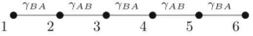
Fig. 1 System corresponding to Hamiltonian in Eq. (13) forn=6. Each node corresponds to qubits in the system and the edges to a two-body interaction

We start by defining the cost and driver Hamiltonians in a one-dimensional line as in [15],

HZ =

j

ωAZ2j +ωBZ2j+1+γA BZ2jZ2j+1+γB AZ2j+1Z2j+2

=ωAHA+ωBHB+γA BHA B+γB AHB A, (13) HX =

j

Xj. (14)

We shall prove that when the number of qubitsnis odd, the QAOA defined with the previous Hamiltonians is universal. For then even case, we will see this is not the case. A graph representing the HamiltonianHZ forn =6 is shown in Fig.1.

For clarity, we make explicit the limits of the sums for each term inHZ. Furthermore, we write in the upper limits of the sums the corresponding limits forneven|nodd.

HA=

n 2|ⁿ⁻₂¹

j=1

Z2j, HB =

n 2−1|ⁿ⁻₂¹

j=0

Z2j+1, (15)

HA B=

n 2−1|ⁿ⁻2¹

j=1

Z2jZ2j+1, HB A=

n 2−1|ⁿ⁻2³

j=0

Z2j+1Z2j+2, (16)

HX = n

j=1

Xj. (17)

It will also be useful to define

Xodd =

n 2−1|ⁿ⁻₂¹

j=0

X2j+1, Xeven=

n 2|ⁿ⁻₂¹

j=1

X2j. (18)

To prove the universality on this model, we shall prove that all one-qubit Pauli operators are in the Lie algebra{i HZ,i HX}Lie, which implies that all one-qubit gates can be generated as consequence of Proposition1. We will also prove that the CNOT gate can be generated by elements in the Lie algebra. With this, we conclude that any unitary can be generated with enough depth on the QAOA sequence. This proves the existence of such QAOA sequence but does not give a particular set of angles to obtain the unitary, neither will we study the efficiency of the method which we leave as an

open problem for future work. We will start by proving the following lemma which allows to separate the quadratic and linear terms onHZ.

Lemma 1 i HZ1=ωAi HA+ωBi HB∈L= {i HZ,i HX}Lie. Note that as a conse- quence, we have that i HZ2=γA Bi HA B+γB Ai HB A∈L

Proof Consider first the commutator

HY Z = 1

2i[HZ,HX] =ωA

n 2|ⁿ⁻2¹

j=1

Y2j +ωB

n 2−1|ⁿ⁻2¹

j=1

Y2j+1

+γA B

n 2−1|ⁿ⁻¹2

j=1

(Y2jZ2j+1+Z2jY2j+1)

+γB A

n 2−1|ⁿ⁻³2

j=0

(Y2j+1Z2j+2+Z2j+1Y2j+2),

(19)

and then, let us perform the calculation

1

2i[HY Z,HX] = −ωA

n 2|ⁿ⁻2¹

j=1

Z2j −ωB

n 2−1|ⁿ⁻2¹

j=1

Z2j+1

+γA B

n 2−1|ⁿ⁻¹2

j=1

2(Y2jY2j+1−Z2jZ2j+1)

+γB A

n 2−1|ⁿ⁻³2

j=0

2(Y2j+1Y2j+2−Z2j+1Z2j+2),

(20)

and define

H₍1) = 1

2i[HY Z,HX] +HZ

=2γA B

n 2−1|ⁿ⁻2¹

j=1

Y2jY2j+1+2γB A

n 2−1|ⁿ⁻2³

j=0

Y2j+1Y2j+2

−γA B

n 2−1|ⁿ⁻¹2

j=1

Z2jZ2j+1−γB A

n 2−1|ⁿ⁻³2

j=0

Z2j+1Z2j+2.

(21)

Next, define also

H₍2)= 1

2i[H₍1),HX]

= −3γA B

n 2−1|ⁿ⁻₂¹

j=1

(Y2jZ2j+1+Z2jY2j+1)

−3γB A

n 2−1|ⁿ⁻2³

j=0

(Y2j+1Z2j+2+Z2j+1Y2j+2).

(22)

Finally, notice that we have 1 2i

HY Z +1

3H₍2),HX

=HZ2. (23)

Thus, we find that i HZ2 ∈ L and we can subtract this from i HZ, implying that i HZ1∈L, which completes the proof.

Next, we prove that it is possible to generateXevenandXodd

Proposition 2 Letω²_A=ω²_B, then i Xeven, i Xodd∈L= i HZ,i HXLie

Proof From Lemma1, we have thati HZ1=ωAi HA+ωBi HB,i HZ2=γA Bi HA B+ γB Ai HB A∈L.

Next, let us define the following element in the Lie algebra HY1= 1

2i[HZ1,HX]

=ωA

n 2|ⁿ⁻₂¹

j=1

Y2j+ωB

n 2−1|ⁿ⁻₂¹

j=0

Y2j+1,

(24)

and then calculate the commutator 1

2i[HZ1,HY1] =ω²_A

n 2|ⁿ⁻₂¹

j=1

X2j+ω²_B

n 2−1|ⁿ⁻₂¹

j=0

X2j+1. (25)

Now notice that

ω²_AHX−ω²_A

n 2|ⁿ⁻₂¹

j=1

X2j −ω²_B

n 2−1|ⁿ⁻₂¹

j=0

X2j+1=(ω²_A−ω²_B)

n 2−1|ⁿ⁻₂¹

j=0

X2j+1, (26)

which implies that ifω²_A=ω²_B, theni Xeven,i Xodd∈L.

From what we have so far proved, we can then generateHA,HB,HA B,HB A. The following proposition states the conditions for this.

Proposition 3 Assumeγ_{A B}² =γ_{B A}² and letγ =(γ_{A B}² −4γ_{B A}² ). Ifγ =0,γ_{A B}² =0, γ_{B A}² =0, then i HA, i HB, i HA B, i HB A∈ i HZ,i HXLie.

The proof of Proposition3is given in “Appendix A”. Note that in Ref. [15] it was required thatωA, ωB, γA B, γB Abe rationally independent. In our proof of universality, this will be relaxed to the condition given by Proposition3.

In the following, we will prove that whennis odd and the condition of the previous lemmas and propositions is fulfilled, QAOA can implement all one-qubit operators andC N O T.

Lemma 2 Assuming n is odd, then i Xj ∈ i HA,i HB,i HA B,i HB A,i HXLiefor any j∈ {1, . . . ,n}.

The proof of Lemma2is given in “Appendix A”.

Theorem 1 Given an odd integer n, HZ as in Eq.(13), HXas in Eq.(14), with coeffi- cients in HZand HXfulfilling the conditions of Proposition3andL= i HZ,i HXLie, then e^Lis dense inU(n). This implies universality for odd integers in QAOA.

Proof We proved in Lemma2that RX(θ) = e^i2Xθ ∈ e^Lit is easy to see that also RY(φ),RZ(ψ) ∈ e^L. Thus, all single qubit operators are ine^L. If it is possible to generate a two qubit gate such asC N O T, then we can prove thatLcan generate any unitary by, for example, generating the gate set of Clifford gates +T, which are known to be universal for quantum computation. In fact, any two-qubit entangling operator with all one-qubit gates is enough for universality [24].

In the proof of Lemma2, we have managed to generate not only one-qubit Pauli’s but also two-qubit Pauli’s such asZk−1Zk. To see thatC N O Tgates can be generated, recall thatC N O T = |00| ⊗1+ |11| ⊗X =¹₂(1⊗1+Z⊗1+1⊗X−Z⊗X).

Note that this last expression is inL.

Finally, note that

e^{iπ4(1⊗1−1⊗X−Z⊗1+Z⊗X)}=e^{iπ4(1−1⊗X)(1−Z⊗1)}

=C N O T. (27)

Since1⊗1−X2−Z1+Z1X2is inL, we conclude thatC N O Tcan be generated.

With this, we have proved universality forn odd. It is easy to see that forneven i HZ,i HXLiecannot approximateU(2ⁿ)due to the presence of a symmetry in the system. This is easier to see with a concrete example, ifn=4 and we number qubits from 1 to 4 then exchanging qubit 1 with qubit 4 and exchanging qubit 2 with qubit 3 is a symmetry of the system. The presence of a symmetry in HamiltoniansHZ and HX implies non-universality; letU be the unitary implementing the symmetry com- muting with both Hamiltonians; then,HZ andHXcan be block diagonalized, which necessarily implies that there are elements inU(2ⁿ)that cannot be approximated. Note nonetheless that forneven, we can just add an extra qubit to obtain universality.

(a) Step 0 (b) Step 1 (c) Step 2

(d) Step 3 (e) Step 4 (f) Step 5

Fig. 2 Example of a zero forcing process on a graph. The initial set of infected verticesSis shown in red in (a); the rest of nodes are uninfected initially. At any step, a given node that has a unique non-infected neighbour infects such neighbour. At each step, we color red the corresponding infected nodes (Color figure online)

4 Universality for QAOA defined on graphs

In Sect.3, we prove universality in a particular setting of a QAOA. Here, we show that universality can be obtained also in more general settings. The algorithms defined here are characterized by the choice of the HamiltoniansHZ andHX. To defineHZ, we make a correspondence between a non-directed simple graph (no loops or multiple edges) G = (V,E)and the terms appearing in HZ, while the Hamiltonian HX is defined as in Sect.3.

4.1 Universality from zero forcing

We prove in this section that the property of universality on this class of QAOA is present depending on a process defined on the graphGcalled zero forcing. The notion of zero forcing has been presented before in the context of quantum control on graphs [29,30,42], and we find that it applies as well in this context.

Definition 3 (Zero forcing) Consider a simple graph G = (V,E), a zero forcing process onGconsists of an initial set of verticesS ⊆V which we will consider as

“infected”. The rest of the vertices are non-infected. Then, we proceed by steps to infect other nodes; at each step, an infected vertexvinfects a non-infected neighbour wifwis the only non-infected neighbour ofv. We callSa zero forcing set if we can infect all the graphs by starting with all infected vertices inS.

An example of a zero forcing process is shown in Fig.2. As usual with QAOA, we start defining two HamiltoniansHZ andHX. Consider simple graphG=(V,E)and a subsetS ⊆V.

HZ =γ

(i,j)∈E

ZiZj +

i∈S

ωiZi +ω

i∈V\S

Zi

=γH_γ +

i∈S

ωiZi +ωHV, (28)

HX =

i∈V

Xi. (29)

Theorem 2 Let G = (V,E) be a simple graph and S ⊆ V . Define HZ and HX

as in Eqs.28and29and letγ,ωi,ωbe rationally independent. Consider S as the initial set of infected nodes in a zero forcing process. If S is a zero forcing set, then ZkZj ∈ HZ,HXLiefor all(k,j)∈ E and Xk ∈ HZ,HXLiefor all k∈V . Proof Sinceγ,ωi,ωare rationally independent, using a similar method to the proof in Proposition 4(see “Appendix B”) we can generate H_γ,HV,Zi fori ∈ S. First, note that for verticesi ∈ Swe can generateXi. Consider two verticesi,j ∈S such that they are neighbouring vertices inG. To see this, commute

1

(2i)²[[H_γ,Xi],Xj] =YiYj. (30) Thus, we can also generate ZiZj. Consider nowi ∈ S that only has one neighbour j∈V\S. We show that we can generateXj. DefineHiasH_γwith the interaction terms corresponding to infected neighbours ofisubtracted. Consider now the commutator:

1

2i[Xi,Hi] =YiZj. (31)

And thus,ZiZj can be generated. Then, we can commute withHX−Xi and generate ZiYj which commuted with ZiZj generates Xj. This is analogous to an infection step in the zero forcing process. It is then easily seen that ifSis zero forcing, then all one-qubit and two-qubit operators are generated in the graph.

We can generalize even more this zero forcing process by difference considering edge interactions in HZ. Given once again a graph G = (V,E)and set S ⊆ V, consider now that we can partition the set of edgesEintoqdisjoint sets{Ei}i∈[q]such that

i∈[q]Ei =E. From this, we write the Hamiltonian HZ =

q k=1

(i,j)∈Ek

γkZiZj+

i∈S

ωiZi+ω

i∈V\S

Zi

= q k=1

γkH_γk+

i∈S

ωiZi+ωHV.

(32)

Definition 4 (Generalized zero forcing for multi-type edges) Consider a simple graph G =(V,E)withE =

i∈[q]Ei, a zero forcing process onGconsists of an initial set of verticesS ⊆V which we will consider as “infected”. The rest of the vertices are non-infected.

The generalized zero forcing process proceeds in one step by considering each infected vertex and the subgraphG1 = (V,E1). If an infected vertex has a single non-infected vertex inG1, then infect this new vertex and add it toS. Then, proceed

in the same fashion with the neighbours of vertices onSin graphsG2,G3, . . . ,Gq. Repeat this process, and if the whole graph ends infected, then we call the initial set Sa generalized zero forcing set.

We prove the following result.

Theorem 3 Let G=(V,E)be a simple graph, S⊆V and consider a partition of the set of edges E into q disjoint sets{Ei}i∈[q]such that

i∈[q]Ei =E. Define HZ and HX as in Eqs.(32)and(29)and letγ,ωi,ωbe rationally independent. Consider S as the initial set of infected nodes in a zero forcing process. If S is a generalized zero forcing set, thenHZ,HXgenerates ZkZjfor all(k,j)∈E and Xkfor all k∈V . Proof The proof is almost the same as in Theorem2.

4.2 Universality without zero forcing

Note that a Hamiltonian defined from a graph and an initial subset of verticesSmay not have a zero forcing set, yet nonetheless can be universal. We will give one such an example with a two-dimensional grid with only two edges under control, meaning that the coupling constant for linear and quadratic terms of the Hamiltonian including the edges and nodes in control is different than for the other terms in the Hamiltonian.

This example points to a more general process than zero forcing that allows to study universality in the corresponding QAOA, although we will not pursue this direction in this work.

Define a graph composed of a square grid withN =n²vertices, number the vertices fromv1tovNleft to right and top to bottom . We assume all interactions in the grid are labelled by the same interaction type A. We also add two extra nodes labelledvN+1

andvN+2. ConnectvN+1to vertexv1with an edge labelled Band connectvN+2to vN with an edge labelledC. We give an example forN =25 in Fig.3.

For this graph, we define the following Hamiltonians:

HZ =ωA

vi∈V_{Gr i d}

Z_vi +ωBZ_vN+1+ωCZ_vN+2 +γA

(vi,vj)∈E_{Gr i d}

Z_viZ_vj +γBZ_v1Z_vN+1+γCZ_vnZ_vN+2, (33)

HX =

N+2 i=1

Xi. (34)

We want to prove that every one-qubit operatorZi and two body operators ZiZj

can be generated.

Note that Lemma1applies in this situation as well, so we can separate HZ1=ωAHA1+ωBZN+1+ωCZN+1,

HZ2=γAHA2+γBZ_v1Z_vN+1+γCZ_vnZ_vN+2.

Fig. 3 Grid withN=25 nodes which defines a Hamiltonian as in Eq. (33). Vertices 26 and 27 correspond to qubits whereH_Z acts with one-qubit operators with coefficientsωBandωC, the corresponding incident edges define two-qubit interactions with coefficientsγBandγC (color online)

1 2 3 4 5

6 7 8 9 10

11 12 13 14 15

16 17 18 19 20

21 22 23 24 25

26 27

From this, we easily see that we can generate as well XN+1, XN+2and XGr i d = _N

i=1Xi. Finally, notice that generatingHA1,ZN+1,ZN+1,HA2,Z_v1Z_vN+1,Z_vnZ_vN+2 separately can be done by applying Proposition4.

To prove that any gate can be generated with these Hamiltonians, we prove that all Zj with j ∈ {1, . . . ,n}andZkZk+1withk ∈ {1, . . . ,n−1}can be generated.

In this way, there is full controllability of the first horizontal line in the grid. After proving this, it directly follows that QAOA defined from the grid is universal by the zero forcing argument.

Theorem 4 Given a graph G as described above, vertices numbered in the order mentioned previously, and given the Hamiltonians HA1, ZN+1, ZN+2, XN+1, XN+2, XGr i d, HA2, Z1ZN+1, ZnZN+2, then for i ∈ {1, . . . ,n−1}and j ∈ {1, . . . ,n}we have that Zj, Xj ,ZiZi+1∈ HA1, ZN+1, ZN+1, HA2, Z1ZN+1, ZnZN+2Lie. This implies universality for any n on the grid.

The proof is given in “Appendix C”. As mentioned before, this points to a more general process that allows to show universality but for brevity we will not go further in this direction.

5 Universality for QAOA defined on hypergraphs

So far, the HamiltoniansHZ induced by graphs define only quadratic or linear terms.

We can consider higher-order terms for HZ by studying a modified version of a zero forcing process on hypergraphs. Here, we will consider the specific case of Hamilto- nians with cubic terms as there is already work studying problems with cubic-order term Hamiltonians as in the MAXE3LIN2 problem [43].

From a hypergraph, we can define Hamiltonians HZ withk-body terms where k>2. A hypergraphG =(V,E)is a generalization of a graph, and it is defined by a finite set of verticesV and a finite set E which contains non-empty subsets ofV which are called hyperedges. In Fig.4, we show an example of a hypergraph defined byV = {v1, v2, . . . , v6}and

Fig. 4 Example of a 3-uniform hypergraph on a line where by definition every hyperedge contains three edges (color online)

v1 v2 v3 v4 v5 v6

E =

{v1, v2, v3},{v2, v3, v4},{v3, v4, v5},{v4, v5, v6}

.

This is also an example of a 3-uniform hypergraph; ak-uniform hypergraph is one where all hyperedges have exactlyknodes.

We will prove here universality on 3-uniform hypergraphs with a small modification in the Hamiltonian defined from the hypergraph. Consider a hypergraphG=(V,E) withV = {1, . . . ,n}andE=

{1,2},{1,2,3},{2,3,4}, . . . ,{n−2,n−1,n}

. An example forn =6 is shown in Fig.4(without the 2-edge).

FromG, we define the following Hamiltonians HZ =δ

{i,j,k}∈E

ZiZjZk+γZ1Z2+ω1Z1+ω

i=1

Zi

=δH_δ+γZ1Z2+ω1Z1+ωHV, (35) HX =

i∈V

Xi. (36)

We wish to generate all two-qubit operators between neighbours and one-qubit operators on every vertex. This hyper-zero forcing is defined by starting with some initial set of infected verticesS1and a set of infected 2-edgesS2; at each step, pick an infected vertex; if it has only one non-infected 3-neighbour, then infect the neighbour.

If it has two infected 3-neighbours, share a 2-edge and then connect each infected node to the non-infected one with 2-edges.

In the 3-uniform hypergraph, the infection step in terms of the commutators pro- ceeds as follows: first note that the termZ1Z2Z3can be separated from the other cubic terms and thatX2can be easily separated; now consider

1

2i[Z1Y2,Z1Z2Z3] =X2Z3. (37) From this, we see thatX3can be separated and we can proceed to separateZ2Z3Z4. In this way, we proceed until the end of the chain having produced all one-qubit and two-qubit operators between neighbours which proves universality.

We can define a hyper-zero forcing procedure on hypergraphs which allows to check whether the corresponding QAOA is universal. We will write here for conciseness only the case of hypergraphs with hyperedges with at most three elements although a more generalized version is possible

Definition 5 Consider a hypergraphG=(V,E)where|e| ≤3 for alle∈ E; a hyper- zero forcing process onGconsists of an initial set of verticesS1 ⊆V and an initial

set of 2-edgesS2which we will consider as “infected”. The rest of the vertices and 2-edges are non-infected. Then, we proceed by steps to infect other nodes; at each step, a pair of infected verticesv1, v2infects a non-infected 3-neighbourwifwis the only non-infected 3-neighbour ofv1andv2and also the 2-edgev1, v2is infected. We callS1andS2hyper-zero forcing sets if we can infect all the graphs by starting with S1andS2infected.

An analogous theorem can be derived as in the zero forcing case for relating hyper- zero forcing processes and universality. Here, for simplicity, we state such theorem for hypergraphs with hyperedges containing three or less vertices.

Theorem 5 LetG = (V,E)be a hypergraph with|e| ≤, S1 ⊆ V and S2 a set of 2-edges. Define HZ and HX as in Eqs.35and 36and let all coefficients in HZ be rationally independent. Consider S1as the initial set of infected nodes and S2as the set of infected edges in a hyper-zero forcing process. If S1and S2are hyper-zero forcing sets, then ZkZj ∈ HZ,HXLie for all(k,j) ∈ E and Xk ∈ HZ,HXLie for all k∈V .

Proof Proof follows directly from arguments in the 3-uniform hypergraph case and

similarly as in the zero process case.

In a previous work [26], it was shown that local unitaries and unitaries generated by three-body Pauli operators do not give rise to universality. This directly implies the following no-go result:

Theorem 6 Define HZ and HXas in Eqs.35and36. If the coefficientγin HZis zero, then the QAOA defined by HZ and HXdoes not yield a universal gate set.

6 Conclusion and outlook

We proved the universality of different QAOA set-ups. In particular, we completed an earlier proof of computational universality for a specific set-up given in Ref. [15] and also found two new broad classes of driver Hamiltonians that allow the corresponding QAOA unitaries to approximate any unitary. The first class consists of Hamiltonians with quadratic and linear terms; the quadratic terms are distributed according to the adjacency matrix of a graph, while the coupling strength of the linear terms is grouped into two parts defined by a so-called zero forcing set of the graph. This construction was then generalized to obtain a second class of driver Hamiltonians with higher- order terms corresponding to hypergraphs and generalized zero forcing sets. Here, it should also be mentioned that the square grid example, presented in Sect.4.2, points to a more general graph process different from zero forcing that may further advance an understanding of universality in QAOA circuits (and perhaps also in more gen- eral quantum control set-ups). Another important generalization of our results would be to regard other mixer Hamiltonians and then the type HX =

iXi considered here, e.g. one could considerX Y mixers [35,44]. One could hope to determine more general conditions for universality of QAOA unitaries, which could include the above- mentioned generalizations; we leave this for future work. Such general results could