Comparison of Different Neural Networks Models for Identification of Manipulator Arm Driven by Fluidic Muscles
Monika Trojanová, Alexander Hošovský
Technical University of Košice, Faculty of Manufacturing Technologies,
Department of Industrial Engineering and Informatics, Bayerova 1, 080 01 Prešov, Slovak Republic, email: monika.trojanova@tuke.sk; alexander.hosovsky@tuke.sk
Abstract: The main subject of the study, which is summarized in this article, was to compare three different models of neural networks (Linear Neural Unit (LNU), Quadratic Neural Unit (QNU) and Multi-Layer Perceptron Network (MLP)) to identify of the real system of the manipulator arm. The arm is powered by FESTO fluidic muscles, which allows for two degrees of freedom. The data obtained by the measurements were processed in Python. This program served as a tool for compiling individual dynamic models, predicting measured data, and then graphically interpreting the resulting models.
Levenberg-Marquardt (LM) was used as the learning algorithm because it is more suitable for learning neural networks than for example, the Gauss-Newton method.
Keywords: pneumatic artificial muscle (PUS); learning algorithm; neural network;
identification; manipulator; fluid muscles; Python
1 Introduction
Automation is currently a highly watched process. By implementing automation into the production process, it is possible to increase work productivity and quality, reduce production costs, or protect employees from working in a hazardous environment [1], [2]. One of the manufacturing activities that can be automated is manipulation. Manipulators can be actuated using various kinds of actuators from electric to hydraulic or pneumatic – in addition to common pneumatic cylinders also pneumatic artificial muscles can be used. The development of the use of pneumatic artificial muscles as one of the atypical forms of propulsion is advancing, where the priority is to achieve the best precision in manipulation. As a result, the system needs to be correctly identified and controlled. [3], [4]
Researchers for many years have been devoted to the development and research of artificial muscles. The static and dynamic properties of the artificial muscle have already been described in several articles, e.g. [1], [5], [6], [7]. By recognizing the characteristics of artificial muscles, it is possible to improve their modeling, which can be realized e.g. using different types of neural networks. This was the case in [8], where a hybrid neuron was used to model PUS. The study of dynamics of systems with certain kinematic configuration driven by PAMs can be found in [9], [10]. In both articles, the authors developed and validated the dynamic model of braided pneumatic muscles (also known as McKibben artificial muscle). The effort of all authors of articles is to shift the boundary of knowledge in the field of artificial muscle modeling and subsequent control.
The main objective is to compare the performance of several approaches to experimental identification of the system using neural network. The system is viewed as a SISO system, where the input variable’s pressure difference between the muscles and the output variable is joint angle. In addition to MLP model, which is a standard NN model, we used also LNU and QNU models in which the performances were not previously tested for PAM-based system identification.
It is precisely the issue of “correct identification of the system” which this article deals with. The paper contains the outputs from the dynamics identification of a specific manipulator arm, which drives fluidized muscles from the producer FESTO. Three types of neural networks were used for the identification process itself, and their compilation and evaluation took place in the Python working environment. The article is formally divided into two basic parts. The first contains theoretical starting points from the areas of PAMs, neural networks and learning algorithms that were used in the experimental part. In the second part of the article are described: the investigated manipulator, the data used for the identification and the resulting models of the individual neural networks. At the end of the article, the different models are evaluated in terms of their effectiveness and possible further orientation in the field of research is outlined.
2 Pneumatic Artificial Muscles
The inventor of Garasiev, of Russian origin, constructed the first pneumatic artificial muscle (PAM) in the beginning of the 20th Century, which consisted of a rubber hose, in several places surrounded by rings. The rings were interconnected with fibers from non-stretchable material. Since the middle of the last century, McKibben artificial muscles have attracted more attention. This very well-known muscle has been designed with the intent of applying it in medical environment [5], [6]. Since the PAMs have many advantages (low weight, acceptable stiffness, high flexibility, etc.), the development of this type of drive continues to advance.
[6]
PAMs work on the principle of changing muscle length when changing the pressure in the muscle. If the muscle is compressed by compressed air, it will shorten from L0 to L, increasing its volume and muscle diameter from D0 to D [7].
This contraction Κ will develop an external tensile force (Figure 1). The resultant tensile force Fm depends nonlinearly on the pressure in the muscle Pm and the contraction (Equation 1) [11]. The contraction is expressed by Equation 2 [12].
) , P ( f
F
m
m
(1)% 100 L )
1 L (
0
(2)Figure 1
Pneumatic artificial muscle [11]
McKibben's artificial muscles have a relatively low lifetime. The causative factor is the dry friction between the fibers and the tube, so the development tries to eliminate this negative factor. The FESTO fluidic muscles used in the investigated system are designed to eliminate the friction between the strands of the muscle.
This is secured by the fact that while the classic artificial muscle has an outer layer, an inner layer and endings [9], [10], the FESTO has joined both layers together.
3 Learning Algorithm and Neural Network Models
Neural networks (NN) allow you to classify or approximate any function using training data. They provide a higher reliability than, for example, expert systems.
While expert systems require specific rules for their activity, neural networks can also work with data that contain uncertainties. The ability of neural networks to learn them is similar to statistics, for example, perceptron is the form of a neuron and is similar to a linear model. Neural networks can be taught based on learning algorithms. One type of learning algorithm - the Levenberg-Marquardt method - was chosen for this experiment. This method is mainly used for a higher number of synaptic weights. Using this learning algorithm, the three following NN models were trained: Multi-Layer Perceptron Network with 1 hidden layer, Linear Neural Unit, and Quadratic Neural Unit. [8], [13]
3.1 Levenberg-Marquardt Learning Algorithm
Levenberg-Marquardt (LM) is one of the basic learning algorithms that is similar to Newton's method. LM is an iterative method combining two other methods - the Gauss-Newton method and the Gradient Descent method. This type of learning algorithm is applied to the function in order to minimize it, the solution being of a numerical nature and is very suitable for learning neural networks. [14]
In the following equations, it is expressed how to proceed from Newton's method to the Gauss-Newton method to the Levenberg-Marquardt algorithm itself. From the Newton method shows that the performance index F(x) is given by Equation 3, where the individual members Ak and gk are given by Equations 4 and 5. [15], [16]
1
k 1 k k k
x x A g (3)
k2
k x x
A F x (4)
kk x x
g F x (5)
If F (x) is the sum of square functions and is given by Equation 6, then the gradient F x of the j-th element has the form of Equation 7 or the general
shape of the gradient F x
in matrix form is given by Equation 8. [16]
N 2i
T
i 1
F x x v x v x
(6)
N
i
j i
j i 1 j
F x x
F x 2 x
x x
(7)
T
F x 2J x v x
(8)
The essence of the method is assembling of the Jacobian J(x), whose general shape is given by Equation 9. [16]
1 1
1 n
n n
1 n
x x
x x
J x
x x
x x
(9)
Next it is necessary to find a Hessian matrix, where k,j-th element of this matrix is expressed by Equation 10 or the general matrix form of the Hessian matrix
2F x
is expressed by Equation 11. If S (x) (Equation 12) is small, then the matrix form of Equation 11 can be adjusted to simpler Equation 13.[16]
2
N i
i
2 i
k, j i
k j i 1 k j k j
F x x x x
F x 2 x
x x x x x x
(10)
2F x 2JT x J x 2S x
(11)
N i
2 i
i 1
S x x x
(12)
2F x 2JT x J x
(13)
If we substitute Equations 8 and Equations 13 into Equation 3, we obtain after Equation 14, which represents the relation for calculating the next element xk+1
with using Gauss-Newton method. [16]
1
T T
k 1 k k k k k
x x J x J x J x v x (14)
The Levenberg-Marquardt algorithm (Equation 15) differs from the Gauss- Newton (GN) method because it also contains a unit matrix I and a coefficient μk. This parameter brings to the LM algorithm an advantage compared to the GN method because the learning rate is determined based on μk value. If μk is high, the solution is not satisfactory, and it is not nearby of the optimal solution, so the learning process is slowed. If μk is small, it means that the values of parameters are approximated to the optimal solution. [16]
1
T T
k 1 k k k k k k
x x J x J x I J x v x (15)
3.2 Linear Neural Unit Model
The essence of the Linear Neural Unit is to find a model of the neuron yn that can identify the linear dependence between inputs ui and real yr outputs. The mathematical model of the LNU is expressed by Equations 16 and 17, where u is the input vector (input), the weight vector is denoted as w and k is the time index.
Error of the neuron e expresses to what extent the model represents the real data.
The equation for calculating this error is given by the difference between real and model data (Equation 18). [14], [17]
n
0 i
i i
n k w u k k
y w u (16)
w u
k w u
k w u
kk u
u w w w k
y 0 0 1 1 n n
n 0 n 1 0
n
(17)
k y
k y
ke r n (18)
3.3 Quadratic Neural Unit Model
The essence of the QNU model is similar to LNU that is to find a model that can identify the functional relationship between inputs and outputs. In this case quadratic dependence is sought. Similar to LNU, the mathematical model of QNU (expressed by Equations 19 and 20) contains a weight vector w, a time index k and a vector col u, that is polynomial. For the neuron error applies the same relationship (Equation 18), where is determined the difference between the real outputs and the model outputs. [14], [17]
k w u
k u k w colu
ky i j
n
0 j
n
0 i
j , i
n
(19)
k u
k u k u
k u
k 1 u k u
k u k u
w w w w k y
2 n
0 0
2 i 0
0 0
n , n j , i 1 , 0 0 , 0 n
(20)
3.4 Multi-Layer Perceptron Network Model
Multilayer Perceptor Network is the last neural network model that has been used to identify the system. This is a well-known network architecture that is characterized by having at least one hidden layer. The base unit - the neuron, which is on the hidden layer, is for this type of network called the perceptron (shown in Figure2). The intrinsic activity of neuron is expressed as xi. Output y is obtained by transforming inputs ui using the activation function φi. [13], [17], [18]
Figure 2
Schema of the perceptron [18]
The two most typical activation functions that are used for MLP networks are a logistic function that is defined at <0; 1> and hyperbolic tangents defined at intervals <-1; 1>. The mathematical formula of the logistic activation function is given by Equation 21 and the hyperbolic tangent by Equation 22. [18]
i
log istic x 1
1 exp x
(21)
i
1 exp 2x tauh x
1 exp 2x
(22)
The MLP network is formed by the parallel interconnection of several perceptrons, and subsequently these neurons are interconnected with the neuron on the output layer. The basic task of the network is the approximation of each nonlinear function. The overall structure of the MLP network with one hidden layer is shown in Figure 3. [17], [18]
Figure 3
Overall structure of the MLP network with one hidden layer [18]
The output of the multilayer perceptron network can be mathematically formulated based on Equation 23 (the inputs uj, the weight of the hidden layer wij, the weight of the output layer wi, the activation function φi and the output y). [17], [18]
M p
i i ij j
i 0 j 0
y w w u
(23) Figure 4 shows the structure of a dynamic MLP network with just 1 hidden layer with n number of perceptrons (or neurons). On the input layer there is an input vector that contains data of a dual kind. The input is the measured data, but since it is a dynamic system, the input also forms the yn data. This type of data is the output of the model from earlier epochs. The sensitivity of each perceptron is expressed by the weight Wi. Within the hidden layer, there are two operations, respectively functions. Synaptic operation is a linear function of the input vector and weights. Somatic operation is a nonlinear activation function given by Equation 24. The output layer contains an output neuron defined by the output data vector y and the weights of this neuron V that form a linear function. [14], [17], [19]1 e 1
2
(24)
Figure 4
MLP dynamic network with one hidden layer [14]
4 System Description
The main object of the study was the manipulator arm system, actuated by two pairs of FESTO fluidic muscles. In the right part of Figure 5 is the real manipulator arm and in the left part is a principal schematic of the main element manipulator. The most basic parts of the system are two pairs of FESTO MAS-20 muscles. The compressed air is supplied to these muscles by FIAC Leonardo compressor. Chain mechanism (sprocket-chain) and a pair of rotary joints serve to desirably deflect the arm with the load. The flow of pressurized air to and out of the muscles is controlled through four MATRIX EPR-50 pressure regulators. The regulators also incorporate built-in sensors, which ensure simultaneous pressure sensing in each of the muscles. The Kubler 3610 incremental sensor is used to measure joint rotation. The control logic signals were processed by the Humusoft MF624 I / O PCI card, and the Matlab and Simulink modules served to control the arm.
Figure 5
Principled scheme of manipulator with PAMs
5 Experimental Part
The main part of the research is an experimental part. Its essence was to obtain data from the real system (manipulator arm with PAMs) that was used in the learning and testing processes. Neural network models and the learning algorithm, which were theoretically supported first, were created in program IDLEX. The output of the experimental part is the individual models, which are subsequently evaluated on the basis of the SSE and fit parameters and also compared to each other. This process served to identify the dynamics of the manipulator arm. At this stage we tried to identify only the dynamics of one of the axes to simplify the dynamic model by eliminating the presence of dynamic coupling between the joints.
5.1 Training and Test Data
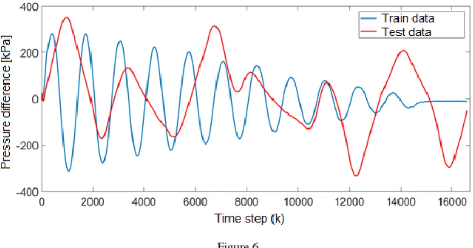
For training and testing of models, measured data were needed. The relationship of interest was between the joint angle (output variable) and pressure difference between the muscles (input variable). A total of 16,667 samples were obtained from one axis of the manipulator arm with a sampling period of 3 ms. The data used in the learning or testing phase has not been sampled (?).
Figure 6 shows the dependence of the pressure difference on the time step used for training and testing. For training (blue curve) the dependence itself has a decreasing character, since triangular excitation signal with a linear decreasing amplitude was used. In this measurement, a pair of muscles was initially pressurized to approximately 300 kPa (i.e. pressure difference was zero). After this the initial set-up, one muscle was discharged, and the other muscle was inflated. For testing (red curve) the data were obtained by generating a random signal with a random amplitude, the curve itself has a random course.
Figure 6
Time dependence of pressure difference for data used in training
5.2 Input Conditions for Models and Individual Models
When compiling individual neural network models in IDLEX, it was necessary to select the input conditions. Using them should ensure the best possible identification of the system. The following parameters were selected for the identification: learning rate μ, number of epochs e, number of inputs nu, number of outputs ny for each model.
A dynamic model with multilayer perceptron network with one hidden layer (MLP) was created, and for this type of network it was also necessary to choose the number of neurons in the hidden layer n1. In Table 1 is show an overview of the entry conditions in which the individual models achieved the best results.
Table 1
Comparison of input conditions for individual models
PARAMETERS LNU QNU MLP
LEARNING RATE 0,05 0,02 0,005
NUMBER OF EPOCHS 4 10 10
NUMBER OF INPUTS U 10 7 10
NUMBER OF INPUTS Y 5 1 5
NUMBER OF NEURONS
ON THE HIDDEN LAYER --- --- 1
For objective model comparison, it is recommended that the number of inputs and outputs be the same for each model. However, the Quadratic Neural Unit model did not work properly under the same conditions as for LNU or MLP. So, for QNU were chosen such initial conditions, where the model worked the most efficiently.
After setting the entry conditions and creating a program, the learning and testing phases followed showing the results of the models and their graphical interpretations in the program. Each of the models is presented with some pictures: 3 figures relate to the learning phase, the other 3 figures to the test phase.
For only the test phase, network weights successful in the learning phase were used. It follows that the graph of the time depending of the pressure difference is depicted in the epoch when the weights were the most suitable.
Figures related to the learning and testing phase show: the first graph shows the time dependence of difference of pressures for real system (blue curve - yr or yr_test) and for the model (green curve – y or y_test). The second graph shows the error between the system and the model (red curve – e or e_test). The third graph shows the Sum Squared Error (SSE or SSE_test) parameter as a function of epoch - the black curve, which expresses the sum of the quadratic errors between the individual data and the diameters of their groups [14].
5.2.1 Linear Neural Unit
Figure 7 graphically interprets the output model of Linear Neural Unit after the learning phase. The picture shows that the LNU model was relatively well taught even in the low number of epochs, as evidenced by the course of the SSE parameter (Figure 9), which has a stable convergence progress. Differences between model and real data can be seen especially at curve vertices where the green curve is unable to reach the position of the blue curve, especially in the negative angles of the joint.
Figure 7 Training LNU
Figure 8 Training LNU – error
Figure 9 Training LNU – SSE
The results of the test phase are graphically interpreted by Figure 10-Figure 12.
While the learning was done on data that had a decreasing character, testing was performed on data with random amplitude, which was reflected in the course of the model. In this case, the difference between the real (blue curve) and the model (green curve) is more pronounced. The SSE_test parameter indicates a wobble.
Figure 10 Testing LNU
Figure 11 Testing LNU – error
Figure 12 Testing LNU – SSE
5.2.2 Quadratic Neural Unit
In Figure 13 is a graphical representation of the Quadratic Neural Unit output model. The model is shown after training. A higher number of epochs was selected for the QNU learning and testing phase, because it is necessary for proper functioning (Figure 15). Training phase based on either the curve of the model or the progress of the SSE parameter that converges does not look the worst.
However, it is not possible to compare this model with LNU and MLP models (they do not have the same initial conditions).
Figure 13 Training QNU
Figure 14 Training QNU – error
Figure 15 Training QNU - SSE
Although for QNU the most appropriate initial conditions were chosen in which the model achieved the highest possible efficiency, the model worked in the test phase worse than the other two models. The SSE_test parameter (Figure 18), like LNU testing, did not have a purely converging course, and when looking at the course of the green curve it is certain that the model was unable to fit the real data very well at a positive angle (above 20 °) (Figure 16). If the QNU model runs with the same initial conditions as LNU and MLP, the SSE parameter itself would have a chaotic divergence course, and the green curve of the model would not be able to approach towards the model in Figure 13, not even the LNU and MLP model.
Figure 16 Testing QNU
Figure 17 Testing QNU – error
Figure 18 Testing QNU - SSE
5.2.3 Multi-Layer Perceptron Network
The last of the investigated and displayed output model was the MLP. Its graphical interpretation along with the course of real data, errors, and SSE parameters during the training phase is shown in Figure 19-Figure 21. The MLP model (similarly as a model LNU) has also learned well. This is evidenced by the course of the green curve towards the blue. The SSE parameter somewhat fluctuate in the first two epochs, but subsequently dropped significantly and converged.
Figure 19 Training MLP
Figure 20 Training MLP – error
Figure 21 Training MLP - SSE
The multilayer perceptual network, during the testing phase (10 epochs), had parameter SSE_test similar to the parameter SSE for the training phase (Figure 24). In the first epoch, the parameter fluctuates, but then there was a significant decrease and convergence of the SSE_test parameter. The curve, like the QNU model, had a problem in reaching angles above 20 degrees, but below this value, the model was very close to real data (Figure 22).
Figure 22 Testing MLP
Figure 23 Testing MLP – error
Figure 24 Testing MLP - SSE
5.3 Comparison of Individual Models
The efficacy of the individual models examined in the experimental part was compared based on the fit parameter. It is a parameter that was calculated by the Matlab program after entering the following command: fit = goodnessOfFit (y, yr, 'NRMSE'), where y are the values determined by the model and yr are real values.
The given command sets the Normalized Root Mean Square Error (NRMSE), which represents the degree of difference between the predicted and the actual model. Equation 25 expresses the mathematical entry of the NRMSE parameter calculation, where x are test data, xref are reference data and fit is a row vector of length i. [20], [21]
xref :,i x :,i fit(i) 1
xref :,i mean xref :,i
(25)
Figure 25 shows individual output models along with real measured data (black curve). The chart also contains a numerically-expressed parameter fit for each
model. As above, it was suggested that models should be compared under the same input conditions (input and output), so the QNU will be evaluated only on the basis of how best it would be worked in comparison with the measured data.
The QNU model, which is represented by the green curve, reached 77.80% in fit.
This means that it can predict with such precision at the given input conditions.
However, the model was not stable and was not the most appropriate for the type of data.
Figure 25
Comparison of output models with real measured data
The MLP model, which is shown in the blue curve, is already comparable to the LNU (red curve) model because it had the same initial conditions. When comparing based on the fit parameter, LNU was better at 82.84%, while MLP reached 81.66%. However, when analyzing the course curves, the MLP network is able to get closer to the top of the measured data than the LNU. Even at negative angles, the MLP is the most accurate in each negative rotation within the three models compared, but in some positive angles, the measured data is exceeded.
Conclusions
Researchers dealing with the modeling, identification and control of pneumatically-powered systems are aware of the highly positive potential due to their use in industry. However, they are constantly confronted with shortcomings;
therefore they need to eliminate it. That is the reason, why the effort to advance in research is not regressing. Several authors have already identified similar systems with using the Gauss-Newton method or Incremental back-propagation algorithm as learning algorithms, and as models using genetic algorithms, and different ARX and NARX models. Similarly, the authors of this article attempt to extend the knowledge in the area of identification of pneumatically-actuated systems by experimentally researches, where are comparing different methods – neural networks (eg, the QNU was little explored for PAM).
The aim of this experiment was to identify the dynamics of the system (manipulator arm powered by fluid muscles FESTO) using the pre-selected learning algorithm and 3 different neural network models. The Python program (or its subsystem IDLEX) was used to identify it. The LNU, QNU, and MLP models show that the data are relatively highly linear dependent. Of these, the best models were MLP and LNU, so it would be useful to test them further. The results also show that the use of QNU to identify this system is not the most appropriate.
Further testing should be performed measuring to obtain a further set of independent data, and verifying the effectiveness of the models on these data.
Another way to verify the effectiveness of models and their reliability is to create them in another program (e.g. Matlab) and compare the results. In this experimentunsampled data were used, since the correlation analysis showed that sampling of data could lead in the loss of data credibility. The correlation analysis was performed simultaneously for both directions of the manipulator arm joint. In the future, it would be advisable to perform a correlation coefficient analysis especially for each direction of rotation of the joint, which would allow a more accurate identification of the joint rotation above 20 ° in the positive direction.
Acknowledgement
The research is supported by a Grant from the Research Grant Agency within the Ministry of Education, Science, Research and Sport of the Slovak Republic and Slovak Academy of Sciences. Number 1/0822/16 Research of Intelligent Manipulator Based on Pneumatic Artificial Muscles with Three Degrees of Freedom; Number 1/0393/18 Research of Methods for Modeling and Compensation of Hysteresis in Pneumatic Artificial Muscles and PAM-actuated Mechanisms to Improve the Control Performance Using Computational Intelligence as well as the EU Structural Funds Project with ITMS code:
26220220103.
References
[1] Kelasidi, E. et al.: A Survey on Pneumatic Muscle Actuators Modeling. In:
International Symposium on Industrial Electronics. June 27-30, 2011, Gdansk: IEEE, pp. 1263-1269
[2] Escobar, F. et al.: Simulation of Control of a Scara Robot Actuated by Pneumatic Artificial Muscles Using RNAPM. Journal of Applied Research and Technology. 2014, Vol. 12, No. 5, pp. 939-946
[3] Piteľ, J. et al.: Pneumatický umelý sval – perspektívny prvok mechatroniky (1). AT&P journal. 2008, Vol. 12, pp. 59-60, ISSN 1336-233X
[4] Piteľ, J. et al.: Pneumatické umelé svaly: modelovanie, simulácia, riadenie.
Košice: Technická univerzita v Košiciach, 2015, p. 275, ISBN 978-80-553- 2164-6
[5] Wickramatung, K. C. et al.: Empirical Modeling of Pneumatic Artificial Muscle. In: Proceedings of the International MultiConference of Engineers and Computer Scientists 2009. March 18-20, 2009, Hong Kong: IMECS 2009, p. 5
[6] Oliver-Salazar, M. A. et al.: Characterization of pneumatic muscle and their use for the position control of a mechatronic finger. Mechatronics. 2017, Vol. 42, pp. 25-40
[7] Doumit, M. et al.: Development and testing of stiffness model for pneumatic artificial muscle. International Journal of Mechanical Sciences.
2017, Vol. 120, pp. 30-41
[8] Song, CH. et al.: Modeling of pneumatic artificial muscle using a hybrid artificial neural network approach. Mechatronics. 2015, Vol. 31, pp. 124- 131
[9] Tang, R. et al.: An Enhanced Dynamic Model for McKibben Pneumatic Muscle Actuators. In: Proceedings of Australasian Conference on Robotics and Automatization. December 3-5, 2012, Wellington, p. 8
[10] Doumit, M. et al.: Analytical Modeling and Experimental Validation of the Braided Pneumatic Muscle. IEEE Transactions on Robotics. 2009, Vol. 25, No. 6, pp. 1282-1290
[11] Chang, M-K. et al.: T-S fuzzy model based tracking control of a one- dimensional manipulator actuated by pneumatic artificial muscles. Control Engineering Practice. 2011, Vol. 19, pp. 1442-1449
[12] Lin, CH-J. et al.: Hysteresis modelling and tracking control for a dual pneumatic artificial muscle system using Prandtl-Ishinskii model.
Mechatronics. 2015, Vol. 28, pp. 35-45
[13] Kvasnička, V. et al: Introduction to the theory of neural networks. Slovakia, Bratislava: IRIS. 1997, p. 237, ISBN 9-788-088-77830-1
[14] Bukovský, I.: Nonconventional Neural Architectures and their Advantages for Technical Applications. Faculty of Mechanical Engineering. Praque:
Czech Technical University in Praque. 2012, ISBN:978-80-01-05122-1 [15] Tomczyk, K.: Levenberg-Marquardt algorithm for optimization of
mathematical models according to minimax objective function of measurement systems. Metrology and Measurement systems. 2009, Vol.
XVI (2009), No. 4, pp. 599-606. ISSN 0860-8229 [16] Hagan, M. T. et al: Neural Network Design. ebook
[17] Nelles, O.: Nonlinear system identification: from classical approaches to neural networks and fuzzy models. Germany. Berlin: Springer. 2001, p.
786, ISBN 3-540-67369-5
[18] Karray, F. O. et al: Soft Computing and Intelligent Systems Design:
Theory, Tools and Applications. England. Harlow: Addison Wesley. 2004, p. 584, ISBN 0-321-11617-8
[19] Haykin, S.: Neural Networks: A Comprehensive Foundation. India:
Pearson Education, 2005, p. 823, ISBN 81-7808-300-0
[20] Rimarčík, M.: Štatistika pre prax. 2007, p. 199, ISBN 978-80-969813-1-1 [21] Ljung, L.: System Identification Toolbox User´s Guide. Natick: The Math
Works, 2015, p. 982