Neural Networks in Bankruptcy Prediction - A Comparative Study on the Basis of the First Hungarian Bankruptcy Model

(1)

NEURAL NETWORKS IN BANKRUPTCY PREDICTION – A COMPARATIVE STUDY ON THE BASIS OF THE FIRST HUNGARIAN

BANKRUPTCY MODEL*

M. VIRÁG – T. KRISTÓF

(Received: 5 March 2005; revision received: 2 July 2005;

accepted: 17 August 2005)

The article attempts to answer the question whether or not the latest bankruptcy prediction tech- niques are more reliable than traditional mathematical–statistical ones in Hungary. Simulation experiments carried out on the database of the first Hungarian bankruptcy prediction model clearly prove that bankruptcy models built using artificial neural networks have higher classification accuracy than models created in the 1990s based on discriminant analysis and logistic regression analysis. The article presents the main results, analyses the reasons for the differences and presents con- structive proposals concerning the further development of Hungarian bankruptcy prediction.

Keywords:solvency, bankruptcy modelling, bankruptcy prediction, discriminant analysis, logistic regression, neural networks

JEL classification index:B41, C15, C45, C53, G33

Forecast methodology is constantly evolving. Significant progress has been made in recent years in the areas of mathematical–statistical, collective expertise and participatory, as well as modelling procedures (Nováky 2001). Findings of the research into artificial intelligence have posed serious challenges to practitioners of mathematical–statistical methods. In Hungary, artificial neural networks of the artificial intelligence family started to gain acceptance after the turn of the millen- nium both in professional literature and in practice; more and more prediction and decision-making modelling problems have recently been solved successfully using such methods. Literature on data mining covers the issue and procedures of ar-

Acta Oeconomica, Vol. 55 (4) pp. 403–425 (2005)

* This article was written as part of the research programme of the HAS-CUoB Complex Futures Studies Research Group (Head of Research Group: Erzsébet Nováky, DSc), operating within the framework of the Hungarian Academy of Sciences and the Corvinus University of Buda- pest.

Corresponding author:M. Virág, Department of Corporate Finance, School of Business Adminis- tration, Corvinus University, Fõvám tér 8, E-350, H-1093 Budapest, Hungary. E-mail:

miklos.virag@uni-corvinus.hu

(2)

tificial intelligence thoroughly (Bigus 1996). These prediction methods have found their way to bankruptcy prediction as well (Kristóf 2004).

Recent empirical studies indicate that neural networks provide a more reliable bankruptcy prediction method than discriminant analysis and logistic regression analysis, used formerly (Atiya 2001; Back et al. 1996; Ooghe et al. 1999). How- ever, based on international experience, the authors reckoned that a comparative study is necessary to see whether international trends prevail in Hungarian bankruptcy models as well.

We hope that the neural network modelling made on bankruptcy prediction will contribute to the promotion of this promising technique in Hungarian professional thinking and also in prediction procedures.

THE FIRST HUNGARIAN BANKRUPTCY PREDICTION MODEL AND ITS HISTORY

Corporate failure prediction has been one of the most interesting financial–statistical challenges. Subjective judgement of solvency is as old as money. Lenders, both individuals and institutions, have always attempted to evaluate whether they will get their money back in the future. Elements of intuitive judgement are still present in today’s credit assessment practice.

There were no sophisticated statistical methods and computers available to pre- dict bankruptcy in the first two thirds of the 20^thcentury. The financial ratios of surviving and bankrupt companies were compared and it was concluded that in case of bankrupt companies the most frequently used debt, liquidity, profitability and turnover ratios were lower, i.e. worse (Fitzpatrick 1932).

Before the 1960s corporate solvency used to be assessed using univariate statistical methods. Beaver (1966) identified thirty financial ratios mentioned frequently in professional literature as relevant to the future solvency of enterprises.

He used univariate discriminant analysis to study the ratios of 79 pairs of solvent/insolvent companies. In his calculations Cash-flow and Total Assets Ratio, which showed insolvency with 90% accuracy one year before actual bankruptcy, gave the best results.

Multivariate discriminant analysis has been applied in bankruptcy prediction since the end of the 1960s. Using this method, Altman (1968) built his world fa- mous bankruptcy model for 33 pairs of solvent/insolvent companies and five financial ratios, which proved to be 95% successful in predicting bankruptcy one year before. Altman, Haldeman and Narayanan (1977) developed their seven- variable ZETA model for 58 solvent and 53 insolvent companies also based on multivariate discriminant analysis.

(3)

In the 1980s, discriminant analysis became more and more replaced and sup- plemented by the logistic regression analysis method, which turned out to be the most frequently used bankruptcy modelling and prediction method until the mid-1990s. Logistic regression analysis for the prediction of corporate insolvency on a representative sample was applied for the first time by Ohlson (1980) for a sample of 105 insolvent and 2058 solvent companies, indicating that insolvent companies represent a much smaller proportion in reality than the solvent ones.

Probit analysis used by Zmijewski (1984) is a milestone in the history of prediction of bankruptcyprobability. The recursive partitioning algorithm (Frydman et al. 1985), another development of the 1980s, depicts the combinations of the different variables and thresholds in a decision-tree model, selecting the relevant ones for prediction.

In Hungary, the legal background for bankruptcy procedures and liquidation procedures was created only in 1991¹– therefore, bankruptcy prediction in Hun- gary has not got a decades-long tradition. The first bankruptcy model was developed by Miklós Virág and Ottó Hajdu (Virág – Hajdu 1996; Hajdu – Virág 2001) based on annual report data for 1990 and 1991, using discriminant analysis and logistic regression. The database serving as the background for the bankruptcy model was provided by the Hungarian Ministry of Finance. Of the 154 processing-industry companies involved in the study, 77 were solvent and 77 were insolvent in August 1992. All companies in the sample had at least 300 employees. 17 financial ratios were considered in the course of developing the model. The present study deals only with the bankruptcy model based on the financial indicators of 1991, as this possessed higher classification accuracy than the other. Let us review the calculation methods used in the ratios(Table 1)together with some basic statistics(Table 2).

DISCRIMINANT ANALYSIS BASED ON 1991 ANNUAL REPORT DATA² Multivariate discriminant analysis simultaneously analyses the distribution of several ratios and creates a classification rule which includes several weighted financial ratios³to combine them into a single discriminant value. A precondition for the selection of the ratios to be used is that correlation between them should be

NEURAL NETWORKS IN BANKRUPTCY PREDICTION 405

1 See Act XLIX of 1991 on bankruptcy procedures, on liquidation procedures and on final set- tlements.

2 Miklós Virág is responsible for discriminant-analysis and logistic-regression-based bankruptcy modelling, while neural-network-based bankruptcy modelling and the comparative analyses were carried out by Tamás Kristóf .

3 The financial ratios are the independent variables in the function.

(4)

Table 1

Calculation methods of financial ratios

Name of ratio Calculation of ratio

Quick Liquidity Ratio (Current Assets – Inventory) / Short-term Liabilities Liquidity Ratio Current Assets / Short-term Liabilities

Cash Funds Ratio (%) (Cash / Total Assets) × 100 Cash-flow and Total Debts Ratio Cash-flow / Total Debts

Current Assets Ratio (%) (Current Assets / Total Assets) × 100

Capital Coverage Ratio (%) [(Invested Assets + Inventory) / Own Equity] × 100 Assets Turnover Ratio Net Sales / Total Assets

Inventory Turnover Ratio Net Sales / Inventory

Accounts Receivable Turnover (days) (Accounts Receivable × 360) / Net Sales Debt Ratio (%) (Liabilities / Total Assets) × 100 Own Equity Ratio (%) (Own Equity / Total Assets) × 100

Solvency Ratio Liabilities / Own Equity

Long-term Loans Covered

Investments (%) (Long-term Loans / Invested Assets) × 100 Short-term Loans Covered Current

Assets (%) (Short-term Loans / Current Assets) × 100 Return on Sales (%) (After-tax profit / Net Sales) × 100 Return on Assets (%) (After-tax profit / Own Equity) × 100 Receivable and Payable Accounts Ratio Accounts Receivable / Accounts Payable

Table 2

Averages and standard deviations of the ratios for solvent and insolvent categories

Financial ratios Averages Deviations

Insolvent Solvent Total Insolvent Solvent Total

Quick Liquidity Ratio 0.47 0.97 0.72 0.23 0.75 0.55

Liquidity Ratio 1.15 2.12 1.63 0.45 1.59 1.17

Cash Funds Ratio (%) 95.58 101.24 98.41 52.60 44.77 48.83

Cash-flow and Total Debts Ratio –0.34 –0.05 –0.20 0.29 0.41 0.38

Current Assets Ratio (%) 0.58 0.63 0.61 0.17 0.17 0.17

Capital Coverage Ratio (%) 73.00 71.00 72.00 39.00 51.00 45.00

Assets Turnover Ratio 56.97 57.39 57.18 20.20 22.60 21.44

Inventory Turnover Ratio 0.15 0.09 0.12 0.23 0.23 0.23

Accounts Receivable Turnover (days) 42.26 27.31 34.78 38.20 22.28 31.26

Debt Ratio (%) –19.00 –3.31 –11.15 15.70 15.10 15.40

Own Equity Ratio (%) –42.50 –3.90 –23.20 71.10 68.14 69.61

Solvency Ratio –0.23 0.07 –0.08 0.30 0.34 0.32

Long-term Loans Coved Investments (%) –0.16 0.0002 –0.08 0.16 0.15 0.16 Short-term Loans Covered Current Assets (%) 0.94 21.39 11.17 23.70 21.25 22.59

Return on Sales (%) 58.29 63.40 60.84 16.50 16.50 16.50

Return on Assets (%) 3.36 6.86 5.11 3.27 8.19 6.24

Receivable and Payable Accounts Ratio 0.43 0.81 0.62 0.22 0.64 0.47

(5)

low – otherwise the newly included ratios would hardy contribute to the increase in the reliability of classification. Another condition is that the ratios should have multi-dimensional normal distribution, and also the co-variant matrices of the groups must be identical. When classifying companies, the financial ratios calculated from the annual report data of the individual companies are to be put into the discriminant function making up the linear combination. By comparing the discriminant values that separate solvent and insolvent companies, one can determine which group a certain company belongs to. The general form of the discriminant function is the following:

Z = w1X1+ w2X2+ … + wnXn, (1) where Z is discriminant value; w_iare discriminant weights; X_iare independent variables (financial ratios); andi = 1,…, nwherenis the number of financial ratios.

Analyses have shown that solvent and insolvent companies in the sample differ from each other mostly in the following discriminant variables:

X1: Quick Liquidity Ratio;

X2: Cash-flow / Total Debts Ratio;

X3: Current Assets / Total Assets Ratio;

X4: Cash-flow / Total Assets Ratio.

The sequence of the ratios listed above indicates their role in distinguishing between the groups, meaning that the Quick Liquidity Ratio is the most discriminant one, followed by the other three variables. The discriminant function for the 1991 data was prepared using these variables.

Z = 1.3566X₁+ 1.63397X₂+ 3.66384X₃+ 0.03366X₄. (2) The criticalZvalue is 2.61612, therefore, if the corresponding financial ratios of the given company are put in the function and give a figure higher than 2.61612, the company is to be classified as solvent, while if theZvalue is lower than the critical value, the company is classified as insolvent.

LOGISTIC REGRESSION BASED ON 1991 ANNUAL REPORT DATA Logistic regression analysis is perfectly suitable for exploring the relationship between explaining variables and the probability of binary (ordinal) answers. This procedure puts a logistic function over the binary (ordinal) data using the method

Zoli, a képletekben a kurziv számok jók?

(6)

of maximum likelihood. Logistic regression selects the model variables using the same method as discriminant analysis. A singleZvalue expressed by the probability of survival of the companies in the sample is attached to weighted independent variables. The advantage of this method is that, unlike discriminant analysis, it neither assumes multi-dimensional normal distribution, nor an invariable variance-covariance matrix. Logistic regression analysis works with non-linear relationships and uses the cumulative logistic function for bankruptcy prediction with the help of the following formula:

Pr (solvent) = e e

e e

Z Z

X X

j j

1 1

0

+ = 0∑

+ ∑

+ +

β β

( )

( ).. (3)

where bjare regression parameters;X_jare independent variables (financial ratios);j = 1 ,.., mwheremis the number of financial ratios.

Empirical studies indicate that solvent and insolvent companies differ from each other the most in these variables (financial ratios):

– X₁: Quick Liquidity Ratio;

– X₂: Return on Sales;

– X3: Cash-flow / Total Debts;

– X4: Current Assets / Total Assets;

– X5: Accounts Receivable / Accounts Payable.

Parameters of the logistic regression function expressing the probability of bankruptcy were the following:

– b0 = 3.432;

– b1 = –10.320;

– b2 = 0.01439;

– b3 = –4.438;

– b4 = –0.02992;

– b5 = 8.170.

However, after having calculated the parameters of the function, the value of the dependent variable of the function (the so-called cut-point value) is still not known. If used for classification, this value yields the best classification accuracy.

After putting the figures into the function every one of the companies will have an accurate value between 0 and 1. In case of the 1991 annual report samples, the cut-point value was 0.525 meaning that companies having a higher value would be classified as insolvent.

(7)

The following table compares the classification accuracy of discriminant analysis and logistic regression analysis (Table 3).The higher classification accuracy of logistic regression analysis is partially due to the fact that no assumptions had to be made regarding the distribution of variables included in this model. The several explaining variables used in this model also favour logistic regression.

The companies included in the sample for the development of bankruptcy prediction models are usually chosen to represent different industries. Evidently, the products made by the different industries have different life cycles and there are differences in the factors of production, in market positions, etc. These differences are also reflected in the corporate-level financial ratios. Thus, the sample of companies greatly influences (ex post) the discriminating ratios in the bankruptcy model, as well as their importance in discrimination. The difference in the new sample needed for the study of the predictive capability (ex ante)of the bankruptcy model will thus depend on the chance of the companies to be chosen as well as on their distribution in the given industry.

To what extent corporate financial ratios reflect the capital structure of the given industry, its revenue and expenditure models is an issue that has been discussed by a number of authors (Platt – Platt 1990). In their study, the authors scru- tinised the impact of changes in corporate financial ratios and industry performance on the possibility of bankruptcy.

Making use of their experience, the possibility of using the so-called industry relative ratio is also worth investigating since this ratio is known to improve the prediction accuracy of bankruptcy models. The industry relative ratio is simply the quotient of the given financial ratio of a company and the industrial mean, which can be calculated as follows:

Table 3

Comparison of the classification accuracies of discriminant analysis and logistic regression (n = 154)

Name Bankruptcy prediction method used

Discriminant analysis Logistic regression

Incorrect solvent (number) 20 12

Incorrect solvent (%) 26.0 15.6

Incorrect insolvent (number) 14 16

Incorrect insolvent (%) 18.2 20.8

Total incorrect (number) 34 28

Total incorrect (%) 22.1 18.2

Classification accuracy (percentage) 77.9 81.8

(8)

(Corporate Ratio)_k,j,t

(Industry Relative Ratio)_k,j,t= —————————————— (4) (Industry Mean Ratio)j,t× 100

wherekis the company;jis the industry;tis the type of ratio.

The denominator is multiplied by 100 in order to adjust the percentage ratios to the scale values over one. As a result, the mean value of an industry relative ratio of a given industry has the value of 0.01 at any given time.

Financial ratios may change with time for a number of reasons. However, the industry relative ratio reflects the reaction of individual companies and the industry to a certain event. The great advantage of the formula is that, in spite of considering the changes over time, it guarantees the mean value of industrial distribution at 0.01, assuming that the variance is constant. This solution – allowing for changes within the industry – decreases the instability of data and may improve the prediction accuracy of bankruptcy models created.

Virág and Hajdu created a model family in 1996 able to indicate bankruptcy dangers early for different sectors and branches of the economy, using discriminant analysis, based on the financial data of nearly 10,000 economic units⁴(Virág – Hajdú 1996). Consequently, financial ratios, together with the related weights of sectors and branches of the economy are available in Hungary, which are the most suitable means for distinguishing between bankrupt and surviving companies within a given sector or branch of the economy. The accuracy of the 1996 bankruptcy model family clearly exceeded that of former models due to the wide range of activities covered.

THE NEURAL NETWORK TRAINING ALGORITHM USED IN THE STUDY

Our initial assumption was that if neural networks – suitable for mapping non-linear relationships as well as recognising samples – are used to classify companies into solvent and insolvent categories, we could get bankruptcy models with accuracy rates higher than those of models based on discriminant analysis and logistic regression analysis. A number of papers have already reviewed major features, the structure and the functioning of neural networks (see e.g. Benedek 2000; 2003;

Kristóf 2002), therefore, in the present study only the learning algorithm used for bankruptcy modelling is discussed in detail.

The most widely known learning algorithm of neural networks is the so-called backpropagation (backwards propagation of error) procedure used for the first

4 No bankruptcy calculations had been made earlier on a sample of this size.

(9)

time by Werbos (1974). In order to train a neural network to perform a task, we must adjust the weight of each unit in such a way that the error between the desired output and the actual output is reduced (Stergiou – Siganos 1996). This process requires that the neural network compute the error derivative of the weights (EW). In other words, it must calculate how the error changes as each weight is slightly in- creased or decreased.

The backpropagation algorithm is easiest to understand if all the units in the network are linear. The algorithm computes eachEWby first computingEA, the rate at which the error changes as the activity level of a unit is changed. For output units,EAis simply the difference between the actual and the desired output. To compute theEAfor a hidden unit in the layer just under the output layer, we first identify all the weights between that hidden unit and the output units to which it is connected. Then we multiply those weights byEAs of the connected output units and add the products. After calculating all theEAs in the hidden layer just under the output layer, we can compute theEAs for other layers in the same way, moving from layer to layer in a direction opposite to the way activities propagate through the network (hence the term “backpropagation”). OnceEAhas been computed for a unit, it is straightforward to computeEWfor each incoming connection of the unit.EWis the product ofEAand the activity through the incoming connection.

In case of non-linear units, the backpropagation algorithm includes an extra step. Before backpropagating,EAmust be converted intoEI, the rate at which the error changes as the total input received by a unit is changed.

The weight of connections is expressed in real figures. Wij stands for the weight of the connection fromi-th unit toj-th unit. It is then convenient to represent the pattern of connectivity in the network by a weight matrix. Two types of connection are usually distinguished: excitatory and inhibitory. Positive weight represents an excitatory connection whereas negative weight represents an inhibitory connection. The pattern of connectivity characterises the architecture of the network. A unit in the output layer determines its activity by following a two step procedure.

(a) First, we must determine the total weighted inputXj, using X_j y W_i _ij

i

=

∑

^, ⁽⁵⁾

whereyiis the activity level of thej-th unit in the previous layer; andWijthe weight of the connection between thei-th and thej-th unit.

(b) Next, the unit calculates the activity yj using some function of the total weighted input. Typically we use the sigmoid function:

(10)

y

j = e X_j

+ ⁻ 1

1 . (6)

Once the activities of all output units have been determined, the network computes the error(E)which is defined by the formula:

E y_i d_i

i

=¹₂

∑

⁽ − ^{) ,}² ⁽⁷⁾

whereyiis the activity level of thei-th unit in the output layer; anddiis the desired output of thei-th unit.

The backpropagation algorithm consists of four steps:

(Step 1) It computes how fast the error changes as the activity of an output unit is changed. This error derivative(EA)is the difference between the actual and the desired activity.

EA E

y y d

j j

= ∂ = −

∂ . (8)

(Step 2) It computes how fast the error changes as the total input received by an output unit is changed. This quantity(EI)is the result of (step 1) multiplied by the rate at which the output of a unit changes as its total input is changed.

EI E

x E y

y

x EA y y

j

j j

j j j

= ∂ = × = −

∂

∂ (1 ). (9)

(Step 3) It computes how fast the error changes as a weight on the connection into an output unit is changed. This quantity(EW)is the result of (step 2) multiplied by the activity level of the unit from which the connection ema- nates.

EW E

W E x

y

W EI y

ij

ij j

j ij

j i

= ∂ = × =

∂

∂ . (10)

(Step 4) It computes how fast the error changes as the activity of a unit in the previous layer is changed. This crucial step allows backpropagation to be applied to multilayer networks. When the activity of a unit in the previ-

(11)

ous layer changes, it affects the activities of all the output units to which it is connected. So, to compute the overall effect on the error, we add all these separate effects on output units. Each effect is quite simple to calculate. It is the result of (step 2) multiplied by the weight of the connection to that output unit.

EA E

y

E x

x

y EI W

i

i j

j i

j ij

j j

=_∂^∂ =

∑

_∂^∂ ×^∂_∂ =

∑

^. ⁽¹¹⁾

By Steps (2) and (4),EAs of one layer of units can be converted intoEAs for the previous layer. This procedure can be repeated to getEAs for as many previous layers as desired. Once we knowEAof a unit, we can use steps 2 and 3 to compute EWs on its incoming connections.

The above procedure aims to find the optimum solution by backward propagation of the errors between actual inputs. The method assumes that similar examples are available to the network, and following pattern recognition it searches for the right connections among neurons in order to create the most successful prediction model.

Note that the backpropagation algorithm procedure itself does not necessarily find the global minimum of the error function; it may settle at a local minimum.

Empirical studies show that a neural network of 35 weights could have several thousands of local minimums (Gonzalez 2000: 29). However, a lot of local minimums make a relatively accurate or acceptable prediction possible.

Experience has shown that neural networks give the best results if they are built with the assistance of experts (Shachmurove 2002: 31). Experts can help significantly improve the predictive capabilities of neural networks by selecting the most appropriate neuron structure, monitoring the changes in weights representing the variables during the training process, and interfering in it (supervised learning), as well as by screening out the input variables which are suspiciously in strong sto- chastic relation with each other. In our case, expert participation was needed only when running the training algorithm because, for the sake of comparability, our model was made up with the input variables which had already been used in the first bankruptcy model.

Even a relatively simple neural network contains a large number of weights. In case of small samples the many weights allow for limited freedom, often leading to over-training even if the early stopping procedure is applied (Gonzalez loc.

cit.). Over-training occurs when the network does not learn the general problem, but it learns the features of the given database (Benedek 2000). In order to avoid this, the database should be divided to training and test sets. First training is done on a training set, and then the results the network gets on an unknown test set are

(12)

studied. If the hit accuracy is similar to that in the training set, training could be accepted as successful. However, if significant errors occur on the test set, the network is over-trained.

When using the early stopping procedure, the researcher has to make a number of decisions which will have a significant impact on the prediction results. Such a decision is, for example, dividing the sample into training and test sets. The right proportion of the sets is neither theoretically, nor practically determined, thus in our research we decided to employ the 75–25% allocation, the most frequently used ratio in literature. In the course of training neural networks, determining the number of training epochs constitutes another element of critical importance. This requires a number of simulation tests and continuous monitoring because neither the under-trained nor the over-trained neural networks are suitable for prediction.

Practical predictions have proven that, similarly to other prediction methods, neural networks are never 100% reliable. The reliability of models can be determined by the Mean Square Error (MSE) index calculated during the training process of the networks, and by classification accuracy in percentages of the results derived from putting the original indices into the already completed models. Since the classification accuracy of discriminant analysis and logistic regression were determined by putting the original data back into the models, we may only have a realistic, comparable picture of the results of different bankruptcy models by studying the classification accuracy of neural networks the same way. First, however, let us review the comparative analysis of bankruptcy models, based on international empirical surveys.

INTERNATIONAL COMPARATIVE ANALYSIS OF NEURAL-NETWORK-BASED BANKRUPTCY MODELS

Fortunately, quite extensive literature has accumulated on bankruptcy prediction using neural networks by the 21^stcentury. The common feature in the surveys on bankruptcy prediction analysed and listed below in chronological order is that they all compare several methods. Having studied the results, we can argue that of all the methods known today, neural networks tend to yield the best results. A good comparison of empirical researches is provided by Atiya (2001) as well.

Since our objective is to thoroughly examine the results of different forecast methods, elaborated models for financial institutions and industry firms are also discussed.

Neural networks were first used for bankruptcy prediction by Odom and Sharda (1990). The authors compared the performance of a three-layer backpropagation network with the results of discriminant analysis, using data of 74 com-

(13)

panies from their annual reports, based on Altman’s (1968) five financial ratios.

Odom and Sharda found that the neural network gave better results than discriminant analysis because it worked perfectly in case of companies used for training the network. The trained network was tested further on another 55 companies unknown to the network. Of the 27 insolvent companies, 5 (18.5%) were in- accurately classified among the solvent ones with the neural network method, while 11 (40.7%) companies were incorrectly classified with discriminant analysis.

Tam and Kiang (1992) studied banks for solvency. Bankruptcy prediction was done by discriminant analysis, logistic regression,k-th-nearest-neighbour proce- dure, decision-tree and single-layer neural network, as well as by multi-layer neural network. The multi-layer neural network proved to be the best for a one-year time span, whereas logistic regression gave the best result for a two-year period.

However, the multi-layer neural network clearly outperformed other methods in both the one-year and two-year conditions when they switched to “skip one” from the unchanged sample. Thek-th-nearest-neighbour and the decision-tree methods performed far worse than other procedures.

Salchenberger, Cinar and Lash (1992) compared neural networks to logistic regression. Neural networks performed considerably better than logistic regression regarding their classification accuracy. In an 18-month time span for example, logistic regression gave 83.3–86.4% accuracy depending on the threshold used, while the neural network reached 91.7% accuracy.

Coats and Fant (1993) compared the results of discriminant analysis and neural networks. Classification accuracy of neural networks was 81.9–95.0%, depending on the time span (from three years to less than one year), while that of discriminant analysis varied between 83.7 and 87.9%.

Kerling and Poddig (1994) used the database of French companies to compare neural networks and discriminant analysis performance for a three-year prediction time span. Neural network gave 85.3–87.7% accuracy, discriminant analysis gave 85.7% accuracy. Kerling and Poddig also tried a number of interaction studies and the early stopping algorithm.

Altman, Marco and Varetto (1994) used neural networks and discriminant analysis for a sample of 1000 Italian companies for a one-year period. Their analysis did not come up with a clear “winner”, though discriminant analysis gave somewhat better results.

Alici (1995) used principal component analysis and self-organising maps to create a neural network structure and to select input elements. Based on his studies on UK companies, neural networks gave 69.6% to 73.7% accuracy, as against that of discriminant analysis (65.6%) and logistic regression (66.0%).

(14)

Leshno and Spector (1996) experimented with a new type of neural network that included cross-conditions and cosinus relations. Depending on the type of network, classification accuracy for a two-year period varied between 74.2% and 76.4%, as compared to the 72% accuracy of linear perceptron network.

Back et al. (1996) used genetic algorithms to select the inputs of multi-layer neural networks. The method was used for one-, two- and three-year periods pre- ceding bankruptcy, and significant improvement was reported compared to discriminant analysis and logistic regression.

Kiviluoto (1996) used self-organising maps with different time spans, based on Finash companies’ annual reports. He got 81–86% accuracy using self-organising maps built on Fisher metrics.

Olmeda and Fernandez (1997) compared neural networks to discriminant analysis, logistic regression and two types of decision-trees on Spanish banks, for different time spans. They got 82.4% accuracy with the neural network, while accuracy of the other methods varied between 61.8% and 79.5%.

Piramuthu, Raghavan and Shaw (1998) developed a novel technique which al- located symbols to the inputs of multi-layer neural networks. They used their method on a sample of Belgian companies, without an indication of the period of time. The new method yielded 82.9% accuracy, while the procedure without the symbols was accurate only in 76.1% of the cases. The same method was used for American banks when the researchers studied the solvency of such institutions for one- and two-year periods. This procedure gave far better results than traditional methods.

Zhang, Hu and Patuwo (1999) compared the performance of logistic regression and neural networks without an indication of the period of time. Using a sample of production companies, they applied a five-layer neural network and multiple in- teractions. They used Altman’s financial ratios for the input neurons of the neural networks, adding current assets/short-term liabilities liquidity ratios. The neural network performed considerably better than logistic regression, with an accuracy of 88.2% as against that of 78.9%.

Tan (1999) compared probit and the three-layer backpropagation network using the sample of 2144 American credit institutions, of which 66 were insolvent.

He studied 13 financial ratios and 4 dummy variables in order to avoid seasonal changes in the ratios. The classification accuracy of probit was 92.5%, while that of the neural network having had 3000 training epochs was 92.2%.

Neophytou, Charitou and Charalambous (2000) developed insolvency prediction models for UK public industrial firms. Their data set consisted of 51 matched pairs of solvent and insolvent UK public industrial firms covering the period 1988–1997. A parsimonious model including three financial variables (profitability, financial leverage and operating cash-flow) was developed based on a uni-

(15)

variate and, subsequently, forward selection and backward elimination logistic regression analysis. The same three variables were used for the development of alternative prediction models using feedforward neural networks. Neural networks achieved the highest overall classification results for all three years prior to insolvency, with an average classification accuracy of 78%. The logit model, although it achieved a lower percentage of overall correct classification (average: 76%) produced slightly lower type I error rates (average: 16%vs.17% in case of neural networks).

McKee and Greenstein (2000) developed a method based on decision-trees and made a one-year prediction using the data of a number of American companies.

Their method proved to be more successful than neural networks and discriminant analysis regarding type II errors, but it was worse regarding type I errors.

Based on the data of 2408 UK construction companies, Yang (2001) developed an early warning system with probability-based neural networks using Bayes’

classification theory and the method of maximum likelihood, and compared the classification accuracy with those of earlier methods. The probability-based neural network yielded a classification accuracy of 95.3%, exceeding those of the backpropagation network (90.9%), logistic regression (88.9%) and discriminant analysis (81.3%).

Yim and Mitchell (2005) examined the performance of discriminant analysis, logistic regression, multi-layer perception and hybrid neural networks on 121 Brazilian industry firms, 29 of which were in financial distress between 1999 and 2000, applying 22 ratios. The most important finding was based on the fact that the best hybrid neural networks were able to provide better results (94.5%) than all other models (between 81.0% and 83.5%) one year before failure.

NEURAL NETWORK BANKRUPTCY MODEL BASED ON 1991 ANNUAL REPORT DATA

International experience shows that a neural network gives the most reliable prediction if the training sample consists of the same number of solvent and insolvent companies. The 1991 database meets this requirement because discriminant analysis works with solvent/insolvent company pairs. Calculations were made based on the entire database provided by the Hungarian Ministry of Finance, including data on 156 companies as against 154 in the first bankruptcy model. The composi- tion of the 156 companies was the following: 2 from mining industry, 10 from iron and metallurgy industry, 54 from engineering industry, 12 from construction industry, 8 from chemical industry, 38 from light industry and 32 from food indus-

(16)

try. Banks and financial institutions have idiosyncratic annual reports; this is why they were not included in the same model.

The input layer consists of the financial ratios of the processing industry companies as continuous variables. The output layer contains a single neuron: the fact of solvency, with 0 indicating insolvency and 1 indicating solvency. The bankruptcy model was made using the financial ratios listed above(Table 1).

The starting point of artificial intelligence models is the division of the total sample to training and test sets. In our research we decided to allocate 75% of the total sample to the training set and 25% was left to the test set, with a random allocation.

Training neural networks – that is to say, determining the weights – can be done using the available software following three alternative strategies: by running a certain number of training epochs as well as by running it until the lowest Mean Square Error (MSE) of the training set or until the lowest MSE of the test set. The number of training epochs needs to be defined in advance in the latter two cases as well, but during the training process those weights will be finalised which prove to be the best for the chosen strategy. In our opinion, the best strategy for prediction is aiming at keeping the test set error at the lowest possible figure, even if in this case the classification accuracy of the starting database is worse than if the training error is kept at the lowest point.

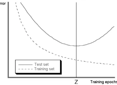
The best way to avoid over-training is to continuously and simultaneously monitor the errors of the training and test sets during the cycles, allowing the network to learn as long as the two errors are close to each other. The number of necessary cycles differs significantly in case the number of neurons differs in the hidden layers(Figure 1).

We were unable to reach a suitably low MSE with a three-layer neural network, no matter what the number of neurons was, which implies an unsuitable predictive capability. Therefore, we continued simulations with four-layer neural networks.

Model experiments showed that it was not worth having less than four neurons in any of the hidden layers because then we got a relatively high MSE value again, which implies a low reliability/accuracy of prediction. The predictive capability of the model also deteriorates if there are more than six neurons in the first hidden layer and more than five in the second hidden layer. The best prediction results were reached when 4–6 neurons were included in the first hidden layer, and 4–5 neurons in the second. In this case the MSE of the test set varied between 7.7% and 17.9%(Table 4).

To establish whether the bankruptcy models are “good” or not, besides MSE, their classification accuracy may also be considered(Table 5). Type I errors arise in case the model incorrectly lists insolvent companies among solvent ones; type II errors occur when the network incorrectly lists solvent companies among insolvent ones.

(17)

Source: Shlens (1999: 5).

Figure 1.Errors of the training and test sets during the training epochs

Table 4

Prediction errors and training epochs of the six neural networks (n=156)

Name Number of neurons in the two hidden layers

4–4 5–4 6–4 4–5 5–5 6–5

Number of training cycles 600 600 1000 1000 1200 1200

MSE (training set) 18.8 17.1 17.1 22.2 17.1 15.4

MSE (test set) 10.3 17.9 12.8 15.4 7.7 7.7

Table 5

Classification accuracy of the training and test sets (n = 156)

Name Number of neurons in the hidden layers

4–4 5–4 6–4 4–5 5–5 6–5

Incorrect solvent (training set, number) 8 3 11 4 9 7

Incorrect insolvent (training set, number) 14 17 9 22 11 11

Total incorrect (training set, number) 22 20 20 26 20 18

Total incorrect (training set, %) 18.8 17.1 17.1 22.2 17.1 15.4 Classification accuracy (training set, %) 81.8 82.9 82.9 77.8 82.9 84.6

Incorrect solvent (test set, number) 1 6 1 5 2 2

Incorrect insolvent (test set, number) 3 1 4 1 1 1

Total incorrect (test set, number) 4 7 5 6 3 3

Total incorrect (test set, %) 10.3 17.9 12.8 15.4 7.7 7.7

Classification accuracy (test set, %) 89.7 82.1 87.2 84.6 92.3 92.3

(18)

Interestingly, all the six models generated more type I errors than type II ones, meaning that neural networks rather tend to classify insolvent companies as solvent than the other way round. The trained four-layer neural network proved to show the highest classification accuracy, thus the most reliable model was the one which had six neurons in the first hidden layer and five in the second one(Figure 2). This network reached 86.5% classification accuracy(Table 6).

In a number of international empirical studies classification accuracy of neural networks was finalised based on the results of the test set, arguing that the predictive capability must be determined on a set completely novel to the network. One could agree with this line of thought – in this case classification accuracy of neural network models would improve significantly in case of 5 nets. Considering, however, that in the cases of discriminant analysis and logistic regression classification accuracy of the models was calculated based on the total input database, we chose to proceed likewise with the neural networks in the present study.

Looking at the classification accuracy, the user might be tempted to accept only the 17-6-5-1-structured four-layer neural network as a final, ready-made model and use this in the future for bankruptcy prediction. However, the practical requirement of multi-variate mathematical statistics also holds for neural networks, i.e. the same observation unit(s) should be processed in as many of the available procedures as possible, and only if similar results are achieved several times can one accept the results.

The results achieved repeatedly prove that based on the particular set of relationships of financial and accounting data and using reliable prediction methods we have a good chance of predicting the future survival of a company.

Also, one must see clearly that the joint use of six models still does not provide 100% reliability in prediction. In the group of solvent companies three, while in the group of insolvent companies six observation units were found to have been

Table 6

Classification accuracy of the six neural networks (n = 156) Name Number of neurons in the hidden layers

4–4 5–4 6–4 4–5 5–5 6–5

Incorrect solvent (number) 9 9 12 9 11 9

Incorrect solvent (%) 11.5 11.5 15.4 11.5 14.1 11.5

Incorrect insolvent (number) 17 18 13 23 12 12

Incorrect insolvent (%) 21.8 23.1 16.7 29.5 15.4 15.4

Total incorrect (number) 26 27 25 32 23 21

Total incorrect (%) 16.7 17.3 16.0 20.5 14.7 13.5

Classification accuracy (%) 83.3 82.7 84.0 79.5 85.3 86.5

(19)

incorrectly classified by all the six models. “Collaboration” among the models can be ruled out because they were all run within different files, and input information was considered randomly in all the learning phases of the models. More probably, the phenomenon may be contributed to the fact that the given company did not carry the signs which could have helped the neural networks recognise them and thus correctly classify the company. A financially seemingly sound and perfect company may go bankrupt because of a single wrong decision made by a man- ager, while others may survive in spite of miserable conditions and bad management.

Further improvement of classification accuracy could only be achieved at the cost of specialising the neural networks for the training database. However, in this case the predictive capability of the models would deteriorate due to over-training already mentioned above.

COMPARISON AND EVALUATION OF THE BANKRUPTCY MODELS CREATED USING DIFFERENT METHODS

If we take classification accuracy as a decisive criterion, neural networks perform better than discriminant analysis and logistic regression, because from the six models five give better accuracy than the 77.9% and 81.8% accuracy achieved by traditional methods. The most reliable neural network of 17-6-5-1 structure is 8.6 percentage points over the classification accuracy of discriminant analysis and ex- ceeds the classification accuracy of logistic regression by 4.7 percentage points.

As for type I error, the neural network outperformed discriminant analysis and logistic regression by 2.8 and 5.4 percentage points, respectively. In case of type II error, neural networks proved to perform 14.5 percentage points better than discriminant analysis, and 4.1 percentage points better than logistic regression.

Besides empirical studies, prediction methodology also helps to prove that neural networks are more successful than discriminant analysis or logistic regression analysis. Discriminant analysis works very well in cases where the variables follow the normal distribution in all groups and the co-variant matrices of the groups are the same. However, empirical studies (e.g. Back et al. 1999) have indi- cated that in particular insolvent companies violate the conditions of normality.

The problems are similar regarding the distribution within the groups. Multi- collinearity among independent variables poses another problem, especially if the stepwise⁵ procedure is employed. Even though empirical studies (e.g. Bern-

5 The stepwise procedure is a regression calculation method that creates the regression function with the smallest square error.

(20)

hardsen 2001) have proven that the lack of normal distribution does not have a negative impact on classification capability, it does affect predictive capability.

The major problem behind discriminant analysis comes from its linearity. Since the discriminant function separates solvent and insolvent groups from each other in a linear way, the ratios within the function will affect classification results always the same way, which does not hold for reality. In spite of the fact that a number of assumptions in the prediction method are not always true, discriminant analysis has been the ruling method in bankruptcy prediction for a long time.

When using logistic regression calculations, it is assumed that the type of function describing the relationship among the variables studied is known in advance and can be described by the logistic curve. However, we know from multi-variate statistics that an incorrectly chosen function leads to an inaccurate estimation of regression coefficients, and thus possibly to bad prediction (Füstös et al. 2004).

Nevertheless, when building neural networks there is no need to go into the type of function describing the phenomenon to be studied, since neural networks can imi- tate any type of functions because of their mathematically proven, so-called uni- versal approximation⁶feature. Therefore, it is not necessary to possess prelimi- nary knowledge for accurate prediction. Neural networks learn the type of relationship from the data themselves, thus minimising the need for information out- side the sample. The use of neural networks is justified exactly by this general ap- proach to functions capability, that is to say, by intelligently finding the relationships between inputs and outputs. This signifies a great advantage in bankruptcy prediction.

The evaluation of the performance of bankruptcy models will not be complete until their predictive capabilities are studied besides the models’ prediction errors and classification accuracy. In order to do so the models need to be tested on actual facts not included in the sample. Consequently, the Hungarian representative neural network based bankruptcy model planned for the near future will be shortly complemented by necessary empirical studies.

SUMMARY

Results achieved using neural networks have shown significant improvement compared to the traditional mathematical–statistical methods. Due to its comparative advantage, neural network modelling should be in the forefront of profes-

6 Cybenko (1989) proved that if a neural network has at least one hidden layer, it is capable of representing an arbitrary number of continuous functions. If the neural network has at least two hidden layers, it is capable of representing an arbitrary number of functions.

(21)

sional attention so as to be used as successfully as possible in Hungarian prediction practice.

The relevance of up-to-date, reliable and high-accuracy bankruptcy prediction models is expected to rise in Hungary in the near future, since after the country’s accession to the European Union competition has been on the increase, conditions are becoming more and more unequal, and thus a relatively high number of bankruptcies are expected. We do not have to go far for examples: after the country’s accession, masses of successful companies with several hundred years of tradition went bankrupt in the neighbouring Austria because German companies with better economies of scale flooded the market.

Hopefully, the results published contribute to convincing Hungarian experts that it is worthwhile to put more financial and intellectual effort into developing a representative, neural-network-based bankruptcy model in Hungary which can handle classification according to activities (economic sectors) as well. Further- more, it would be highly beneficial to carry out detailed research on algorithms even more up-to-date than backpropagation, because there is a lot of yet unex- ploited potential in using neural network modelling for bankruptcy prediction and other ends.

REFERENCES

Act XLIX. of 1991 (1991): Act XLIX of 1991 on Bankruptcy Procedure, on Liquidation Procedure and on Final Settlement.

Alici, Y. (1995): Neural Networks in Corporate Failure Prediction: The UK Experience. In:

Refenes, A. N. – Abu-Mostafa, Y. – Moody, J. – Weigend, A. (eds):Processing Third Interna- tional Conference of Neural Networks in the Capital Markets, London, October:393-406.

Altman, E. I. (1968): Financial Ratios, Discriminant Analysis and the Prediction of Corporate Bank- ruptcy.The Journal of Finance,(23) 4: 589–609.

Altman, E. I. – Haldeman, R .– Narayanan, P. (1977): ZETA Analysis, a New Model for Bankruptcy Classification.Journal of Banking and Finance,(1)1: 29–54.

Altman, E. I. – Marco, G. – Varetto, F. (1994): Corporate Distress Diagnosis: Comparisons Using Linear Discriminant Analysis and Neural Networks.Journal of Banking and Finance,(18)3:

505–529.

Atiya, A. F. (2001): Bankruptcy Prediction for Credit Risk Using Neural Networks: A Survey and New Results.IEEE Transactions on Neural Networks,(12)4: 929–935.

Back, B. – Laitinen, T. – Sere, K. – van Wezel, M. (1996):Choosing Bankruptcy Predictors Using Discriminant Analysis, Logit Analysis, and Genetic Algorithms.Technical Report No. 40. Turku Centre for Computer Science, Turku.

Beaver, W. (1966): Financial Ratios as Predictors of Failure. Empirical Research in Accounting: Se- lected Studies.Journal of Accounting Research, Supplement to Vol. 5: 71–111.

Benedek, G. (2000): Evolúciós alkalmazások elõrejelzési modellekben – I. (Evolution Applications in Prediction Models – I).Közgazdasági Szemle,47(December): 988–1007.

Benedek, G. (2003): Evolúciós gazdaságok szimulációja. PhD értekezés (Simulation of Evolution- ary Economies. Ph.D. Thesis). Budapest: Department of Econometrics and Mathematical Eco- nomics, BUESPA.

(22)

Bernhardsen, E. (2001):A Model of Bankruptcy Prediction. Working Paper. Financial Analysis and Structure Department – Research Department, Norges Bank, Oslo.

Bigus, J. P. (1996):Data Mining with Neural Networks: Solving Business Problems.New York:

McGraw-Hill.

Coats, P. – Fant, L. (1993): Recognizing Financial Distress Patterns Using a Neural Network Tool.

Financial Management,22(3): 42–155.

Cybenko, G. (1989): Approximation by Superpositions of a Sigmoid Function.Mathematics of Con- trols, Signals and Systems, 2(4): 303–314.

Fitzpatrick, P. (1932):A Comparison of the Ratios of Successful Industrial Enterprises with Those of Failed Companies. Washington: The Accountants’ Publishing Company.

Frydman, H. – Altman, E. I. – Kao, D. L. (1985): Introducing Recursive Partitioning for Financial Classification: The Case of Financial Distress.The Journal of Finance,40(1): 303–320.

Füstös, L. – Kovács, E. – Meszéna, Gy. – Simonné Mosolygó, N. (2004): Alakfelismerés.

Sokváltozós statisztikai módszerek(Pattern Recognition. Multivariate Statistical Methods). Bu- dapest: Új Mandátum Kiadó.

Gonzalez, S. (2000):Neural Networks for Macroeconomic Forecasting: A Complementary Ap- proach to Linear Regression Models. Working Paper 2000-07, Department of Finance, Canada.

Hajdu, O. – Virág, M. (2001): A Hungarian Model for Predicting Financial Bankruptcy.Society and Economy in Central and Eastern Europe,23(1–2): 28–46.

Kerling, M. – Poddig, T. (1994): Klassifikation von Unternehmen mittels KNN. In: Rehkugler, H. – Zimmermann, H. G. (eds): Neuronale Netze in der Ökonomie. München: Vahlen Verlag:

424–490.

Kiviluoto, K. (1998): Predicting Bankruptcies with the Self-organizing Map. Neurocomputing, 21(1–3): 191–201.

Kristóf, T. (2002):A mesterséges neurális hálók a jövõkutatás szolgálatában(Artificial Neural Net- works Serving Futures Studies). Jövõelméletek 9. Budapest: Future Theories Centre, BUESPA.

Kristóf, T. (2004):Mesterséges intelligencia a csõdelõrejelzésben(Artificial Intelligence in Bank- ruptcy Prediction). Jövõtanulmányok 21. Budapest: Future Theories Centre, BUESPA.

Leshno, M. – Spector, Y. (1996): Neural Network Prediction Analysis: The Bankruptcy Case.

Neurocomputing,10(1): 125–147.

McKee, T. E. – Greenstein, M. (2000): Predicting Bankruptcy Using Recursive Partitioning and a Realistically Proportioned Data Set.Journal of Forecasting,19(3): 219–230.

Neophytou, E. – Charitou, A. – Charalambous, C. (2000):Predicting Corporate Failure: Empirical Evidence for the UK.Southampton: Department of Accounting and Management Science, Uni- versity of Southampton, 173 pp.

Nováky, E. (2001): Methodological Renewal in Futures Studies. In: Stevenson, T. – Masini, E. B. – Rubin, A. – Lehmann-Chada, M. (eds.):The Quest for the Futures: A Methodology Seminar in Futures Studies. Turku: Finland Futures Research Centre, 187–199.

Odom, M.D. – Sharda, R. (1990): A Neural Network Model For Bankruptcy Prediction. In:Pro- ceeding of the International Joint Conference on Neural Networks, San Diego, 17–21 June 1990,Volume II. IEEE Neural Networks Council, Ann Arbor, 163–171.

Ohlson, J. (1980): Financial Ratios and the Probabilistic Prediction of Bankruptcy.Journal of Ac- counting Research,18(1): 109–131.

Olmeda, I. – Fernandez, E. (1997): Hybrid Classifiers for Financial Multicriteria Decision Making:

The Case of Bankruptcy Prediction.Computational Economics, 10(4): 317–352.

Ooghe, H. – Claus, H. – Sierens, N. – Camerlynck, J. (1999):International Comparison of Failure Prediction Models from Different Countries: An Empirical Analysis.Ghent: Department of Cor- porate Finance, University of Ghent.

(23)

Piramuthu, S. – Raghavan, H. – Shaw, M. (1998): Using Feature Construction to Improve the Per- formance of Neural Networks.Management Science,44(2): 416–430.

Platt, H. D. – Platt, M. B. (1990): Development of a Class of Stable Predictive Variants: The Case of Bankruptcy Prediction.Journal of Business Finance and Accounting,17(1): 31–44.

Salchenberger, L. – Cinar, E. – Lash, N. (1992): Neural Networks: A New Tool for Predicting Thrift Failures.Decision Sciences,23(4): 899–916.

Shachmurove, Y. (2002):Applying Artificial Neural Networks to Business, Economics and Finance.

New York: Departments of Economics, The City College of the City University of New York and The University of Pennsylvania.

Stergiou, C. – Siganos, D. (1996):Neural Networks.Computer Department, Imperial College of London, London. http://www.doc.ic.ac.uk/~nd/surprise_96/journal/vol4/cs11

Shlens, J. (1999):Time Series Prediction with Artificial Neural Networks.Los Angeles: Computer Science Program, Swarthmore College.

Tam, K. – Kiang, M. (1992): Managerial Applications of the Neural Networks: The Case of Bank Failure Predictions.Management Science,38(7): 416–430.

Tan, C. N. W. (1999):An Artificial Neural Networks Primer with Financial Applications Examples in Financial Distress Predictions and Foreign Exchange Hybrid Trading System.Australia:

School of Information Technology, Bond University.

Virág, M. (1996):Pénzügyi elemzés, csõdelõrejelzés(Financial Analysis, Bankruptcy Prediction).

Budapest: Kossuth Kiadó.

Virág, M. – Hajdu, O. (1996): Pénzügyi mutatószámokon alapuló csõdmodell-számítások (Finan- cial Ratio Based Bankruptcy Model Calculations).Bankszemle,15(5): 42–53.

Werbos, P. (1974):Beyond Regression: New Tools for Prediction and Analysis in the Behavioural Sciences.Ph.D Thesis. Cambridge MA: Harvard University.

Yang, Z. (2001):A New Method for Company Failure Prediction Using Probabilistic Neural Net- works.Exeter: Department of Computer Science, Exeter University.

Yim, J. – Mitchell, H. (2005): A Comparison of Corporate Distress Prediction Models in Brazil: Hy- brid Neural Networks, Logit Models and Discriminant Analysis. Nova Economia Belo Horizonte,15(1): 73–93.

Zhang, G. – Hu, M. – Patuwo, B. (1999): Artificial Neural Networks in Bankruptcy Prediction: Gen- eral Framework and Cross-validation Analysis.European Journal of Operational Research, 116: 16–32.

Zmijewski, M. E. (1984): Methodological Issues Related to the Estimation of Financial Distress Pre- diction Models.Journal of Accounting Research,Supplement to Vol. 22: 59–82.