Every hierarchy of beliefs is a type ∗
Mikl´ os Pint´ er
Corvinus University of Budapest
†January 6, 2012
Abstract
When modeling game situations of incomplete information one usually considers the players’ hierarchies of beliefs, a source of all sorts of compli- cations. Hars´anyi (1967-68)’s idea henceforth referred to as the ”Hars´anyi program” is that hierarchies of beliefs can be replaced by ”types”. The types constitute the ”type space”. In the purely measurable framework Heifetz and Samet (1998) formalize the concept of type spaces and prove the existence and the uniqueness of a universal type space. Meier (2001) shows that the purely measurable universal type space is complete, i.e., it is a consistent object. With the aim of adding the finishing touch to these results, we will prove in this paper that in the purely measurable frame- work every hierarchy of beliefs can be represented by a unique element of the complete universal type space.
1 Introduction
It is recommended that the models of incomplete information situations be able to handle the players’ hierarchies of beliefs, e.g. player 1’s beliefs about the parameters of the game, player 1’s beliefs about player 2’s beliefs about the parameters of the game, player 1’s beliefs about player 2’s beliefs about player 1’s beliefs about the parameters of the game, and so on to infinity. The explicit use of hierarchies of beliefs1, however, makes the analysis very cumbersome, hence it is desirable that those should not appear explicitly in the models.
In order to make the models of incomplete information situations more amenable to analysis, Hars´anyi (1967-68) proposes to replace the hierarchies of beliefs by types. There are two approaches to examine the connection be- tween types and hierarchies of beliefs. The first one, when we take a type space as a primitive, in this case each player’s each type in the given type space de- fines a hierarchy of beliefs of the given player (see e.g. Battigalli and Siniscalchi (1999) or the proof of Proposition 18 in Section 4).
∗I thank Ferenc Forg´o, Aviad Heifetz and Zolt´an K´annai for their suggestions and re- marks. Naturally, all errors are mine. This work is supported by the J´anos Bolyai Research Scholarship of the Hungarian Academy of Sciences and by grant OTKA 72856.
†Department of Mathematics, Corvinus University of Budapest, 1093 Hungary, Budapest, F˝ov´am t´er 13-15., miklos.pinter@uni-corvinus.hu
1In this paper we use the terminology hierarchy of beliefs instead of the longer coherent hierarchy of beliefs.
In the second case, we take hierarchies of beliefs first, then we ”construct” a type space of the considered hierarchies of beliefs (see e.g. Mertens and Zamir (1985), Brandenburger and Dekel (1993), Heifetz (1993), Mertens et al (1994), Pint´er (2005) among others). It is an open question in this field whether the two approaches are equivalent, i.e., whether there is a type space containing every hierarchy of beliefs or equivalently whether every hierarchy of beliefs is a type.
Hars´anyi’s main concept is that the types can substitute for the hierarchies of beliefs, and all types can be collected into an object on which the probability measures represent the players’ (subjective) beliefs. Henceforth, we call this method of modeling the ”Hars´anyi program”.
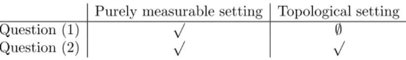
However, at least two questions come up in connection with the Hars´anyi program: (1) Is the concept of types itself appropriate? (2) Can every hierarchy of beliefs be a type?
Question (1) consists of two subquestions. First, can all types be collected into one object? The concept of universal type space formalizes this requirement:
the universal type space in a certain category of type spaces is a type space (a) which is in the given category and (b) into which, every type space of the given category can be ”embedded” in a unique way. In other words, the universal type space is the most general type space, it contains all type spaces (all types).
In the purely measurable framework Heifetz and Samet (1998) introduces the concept of universal type space and proves that the universal type space exists and is unique.
Second, can any probability measure on the object of the collected types (states of the world) be a (subjective) belief? Brandenburger (2003) introduces the notion of complete type spaces: a type space is complete, if its type func- tions are surjective (onto). Roughly speaking, a type space is complete, if each probability measure on the object consisting of the types of the model is as- signed to a type. Meier (2001) shows that the purely measurable universal type space is complete.
We can now conclude that the answer for question (1) is affirmative, i.e., in the purely measurable framework the complete universal type space exists.
Question (2) is whether the universal type space contains every hierarchy of beliefs. Mathematically, the problem is as follows: every hierarchy of be- liefs defines an inverse system of probability measure spaces; the question is the following: do these inverse systems of probability measure spaces have in- verse limits? Kolmogorov Extension Theorem is about this problem, however it calls for topological concepts, e.g. for (inner compact) regular probability mea- sures. Therefore up to now, all papers on this problem, e.g. B¨oge and Eisele (1979), Mertens and Zamir (1985), Brandenburger and Dekel (1993), Heifetz (1993), Mertens et al (1994), Pint´er (2005) among others, use topological type spaces instead of purely measurable ones. Although these papers give a positive answer to question (2), i.e., their type spaces contain all ”considered” hierar- chies of beliefs, very recently Pint´er (2010b) shows that there is no universal topological type space, i.e., there is no topological type space which contains every topological type space, therefore the answer for question (1) is negative in this case, put it differently, in the topological framework the Hars´anyi program fails.
In the above mentioned papers the authors answer question (2) (affirma- tively) by constructing an object consisting of all considered hierarchies of be- liefs, called beliefs space, and show that the constructed beliefs space defines (is
Purely measurable setting Topological setting
Question (1) √
∅
Question (2) √ √
Table 1: The Hars´anyi program equivalent to) a topological type space.
It is worth mentioning that the above papers use different concepts of hi- erarchies of beliefs; e.g. in Mertens and Zamir (1985) the parameter space is a compact topological space, the beliefs are (inner closed) regular probability measures, and the events (for higher order beliefs) are the Borel sets of weak*
topologies, in Brandenburger and Dekel (1993) the parameter space is a Pol- ish space, the beliefs are probability measures and the events (for higher order beliefs) are the Borel sets of weak* topologies, while in Heifetz (1993) the pa- rameter space is a Hausdorff topological space, the beliefs are (inner compact) regular probability measures, and the events (for higher order beliefs) are the Borel sets of weak* topologies, and so on. Therefore, the concept of hierarchy of beliefs is different from paper to paper, from setting to setting.
In this paper we work with the category of type spaces introduced by Heifetz and Samet (1998), i.e., we consider the purely measurable framework (with purely measur-
able type spaces, see Definition 4, and with purely measurable hierarchies of beliefs, see Definition 13). Our main result is that in the purely measurable framework every hierarchy of beliefs is a type, put it differently, the Hars´anyi program works in the purely measurable setting.
The strategy of the proof is the same as in the above mentioned papers on topological type spaces, i.e., we construct an object such that (1) it contains every hierarchy of beliefs (see Definition 13) and (2) it generates a type space.
More exactly, it is showed that the purely measurable beliefs space is equivalent to the purely measurable complete universal type space, we mean those are measurable isomorphic.
As we have already mentioned, the proof that the universal type space con- tains every hierarchy of beliefs is based on the Kolmogorov Extension Theorem.
Since we work in the purely measurable framework, we avoid using topologi- cal concepts, and apply a non-topological variant of the Kolmogorov Extension Theorem. Mathematically speaking, we take a new result of Pint´er (2010a) to show that the inverse systems of probability measure spaces under consideration (the purely measurable hierarchies of beliefs) have inverse limits.
The intuition behind our result is that the purely measurable hierarchies of beliefs are special stochastic processes. No new information enters the process, i.e., the players do not learn anything new (about the states of the world) when they are “thinking“ (considering their hierarchies of beliefs). In general, the hier- archies of beliefs, however, do not have this property, e.g. in Heifetz and Samet (1999)’s example the players can learn new things (about the states of the world) when they are “thinking”.
In our opinion, the purely measurable approach, where the players do not learn anything new about the states of the world, very accurately reflects the intuition that the hierarchies of beliefs are “only“ descriptions of the players’
beliefs. Moreover, this accuracy makes it possible to achieve our positive result.
One important remark: our result does not contradict Heifetz and Samet
(1999)’s counterexample, because their non-type hierarchy of beliefs is not in the purely measurable beliefs space (for details see Section 5).
The paper is organized as follows: Section 2 presents the technical setup and some basic results of the field. Our main result (Theorem 14) comes on stage in Section 3, and in Section 4 we present the proof of Theorem 14. Section 5 is for the detailed discussion of the connection between our result and two other papers Heifetz and Samet (1999) and Pint´er (2010b). The last section briefly concludes. The mathematics of the proof of Theorem 14 is relegated to Appendix A.
2 The type space
Notation: Let N be the set of the players, w.l.o.g. we can assume that 0∈/ N, and letN0⊜N∪ {0}, where 0 is for the nature as a player.
Let #A be the cardinality of setA. For any set system A ⊆ P(X): σ(A) is the coarsestσ-field which containsA. Let (X,M) and (Y,N) be measurable spaces, then (X×Y,M ⊗ N) or brieflyX⊗Y is the measurable space on the set X×Y equipped with theσ-fieldσ({A×B |A∈ M, B∈ N }).
The measurable spaces (X,M) and (Y,N) are measurable isomorphic if there is a bijectionf between them such that bothf andf−1 are measurable.
For any measurable space (X,M) and for any point x ∈X: δx is for the Dirac measure on (X,M) concentrated at pointx.
In the following, we use terminologies that are very similar to Heifetz and Samet (1998)’s.
Definition 1. Let(X,M)be a measurable space and denote ∆(X,M)the set of the probability measures on it. Then the σ-field A∗ on ∆(X,M) is defined as follows:
A∗⊜σ({{µ∈∆(X,M)|µ(A)≥p}, A∈ M, p∈[0,1]}).
In other words,A∗ is the smallest σ-field among theσ-fields which contain the sets {µ ∈ ∆(X,M)| µ(A) ≥ p}, where A ∈ M and p ∈ [0,1] are arbitrarily chosen.
In incomplete information situations it is recommended to consider events like a player believes with probability at least p that a certain event occurs (beliefs operator see e.g. Aumann (1999b)). For this reason, for anyA∈ Mand for anyp∈[0,1]: {µ∈∆(X,M)|µ(A)≥p} must be an event (a measurable set). To keep the class of events as small (coarse) as possible, we use the A∗ σ-field.
Notice that A∗ is not a fixed σ-field, it depends on the measurable space on which the probability measures are defined. ThereforeA∗ is similar to the weak∗ topology, which depends on the topology of the base (primal) space.
Assumption 2. Let the parameter space (S,A)be a measurable space.
Henceforth we assume that (S,A) is a fixed parameter space which contains all states of the nature.
Definition 3. LetΩbe the space of the states of the world and for eachi∈N0: letMibe aσ-field onΩ. Theσ-fieldMirepresents playeri’s information,M0 is for the information available for the nature, hence it is the representative of A, the σ-field of the parameter space S. Let M ⊜ σ( S
i∈N0
Mi), the smallest σ-field which contains allσ-fields Mi.
Each point in Ω provides a complete description of the actual state of the world. It includes both the state of nature and the players’ states of the mind.
The differentσ-fields are for modeling the informedness of the players, they have the same role as e.g. the partitions in Aumann (1999a)’s paper have. Therefore, ifω, ω′∈Ω are not distinguishable2in theσ-fieldMi, then playeriis not able to discern the difference between them, i.e., she believes the same things and behaves in the same way at the two statesω andω′. Mrepresents all informa- tion available in the model, it is the σ-field got by pooling the information of the players and the nature.
For the sake of brevity, henceforth – if it does not make confusion – we do not indicate theσ-fields. E.g. instead of (S,A) we writeS, or ∆(S) instead of (∆(S,A),A∗). However, in some cases we refer to the non-written σ-field: e.g.
A∈∆(X,M) is a set ofA∗, i.e., it is a measurable set in the measurable space (∆(X,M),A∗), butA⊆∆(X,M) keeps its original meaning: Ais a subset of
∆(X,M).
Definition 4. Let(Ω,M)be the space of the states of the world (see Definition 3). The type space based on the parameter spaceS is a tuple(S,{(Ω,Mi)}i∈N0, g,{fi}i∈N), where
1. g: Ω→S isM0-measurable,
2. for eachi∈N: fi: Ω→∆(Ω,M−i)is Mi-measurable,
3. for eachi∈N,ω ∈Ω,A∈ M−i such that there existsA′ ∈ Mi,ω∈A′ andA′⊆A: fi(ω)(A) = 1,
whereM−i⊜σ( S
j∈N0\{i}Mj).
Put Definition 4 differently,Sis the parameter space, it contains the ”types”
of the nature. Mi represents the information available for player i, hence it corresponds to the concept of types (see Hars´anyi (1967-68)). fi is the type function of playeri, it assigns playeri’s (subjective) beliefs to her types.
The above definition of type space differs from Heifetz and Samet (1998)’s concept, but it is similar to the type space of Meier (2001) and Meier (2008).
We do not use a Cartesian product space, and refer only to the σ-fields. By following strictly Heifetz and Samet (1998)’s paper, if one takes the Cartesian product of the parameter space and the type sets, and defines the σ-fields as theσ-fields induced by the coordinate projections (e.g. M0 is induced by the coordinate projectionpr0:S× ×i∈NTi→S, for the notations see their paper), then she gets our concept. However, if the Cartesian product is not used directly, then it is necessary to put the parameter space into the type space in some way.
2Let (X,T) be a measurable space andx, y∈X be two points. xandy are measurably indistinguishable if∀A∈ T: (x∈A)⇔(y∈A).
For doing so we use g (Mertens and Zamir (1985) use a similar formalism), hence g and pr0 have the same role in the two formalizations, in ours and in Heifetz and Samet (1998) respectively.
A further difference between the two formalizations lies in the role of the parameter space. While in Heifetz and Samet (1998) the entire parameter space
”is in” the space of the states of the world, in our approach that is not required.
We emphasize that this difference is not relevant.
Definition 5. The mappingϕ: Ω→Ω′ is a type morphism between type spaces (S,{(Ω,Mi)}i∈N0, g,{fi}i∈N)and(S,{(Ω′,M′i)}i∈N0, g′,{fi′}i∈N)if
1. ϕis anM-measurable mapping,
2. Diagram (1)is commutative, i.e., for eachω∈Ω: g′◦ϕ(ω) =g(ω), Ω
Ω′ ϕ
❄ g′
✲ S g
✲
(1)
3. for eachi∈N: Diagram (2) is commutative, i.e., for eachi∈N,ω∈Ω:
fi′◦ϕ(ω) = ˆϕi◦fi(ω),
Ω fi ✲ ∆(Ω,M−i)
Ω′ ϕ
❄ fi′
✲ ∆(Ω′,M′−i) ˆ ϕi
❄
(2)
where ϕˆi : ∆(Ω,M−i) → ∆(Ω′,M′−i) is defined as follows: for all µ ∈
∆(Ω,M−i), A∈ M′−i: ϕˆi(µ)(A) =µ(ϕ−1(A)). It is a slight calculation to show thatϕˆi is a measurable mapping.
ϕ type morphism is a type isomorphism, if ϕ is a bijection and ϕ−1 is also a type morphism.
The above definition is practically the same as Heifetz and Samet (1998)’s, hence all intuitions, they discussed, remain valid, i.e., the type morphism assigns type profiles from a type space to type profiles in an other type space in the way the corresponded types induce equivalent beliefs. In other words, the type morphism preserves the players’ beliefs.
The following result is a direct corollary of Definitions 4 and 5.
Corollary 6. The type spaces based on the parameter space S as objects and the type morphisms form a category. LetCS denote this category of type spaces.
Heifetz and Samet (1998) introduce the concept of universal type space.
Definition 7. The type space(S,{(Ω,Mi)}i∈N0, g,{fi}i∈N)is a universal type space, if for any type space(S,{(Ω′,M′i)}i∈N0, g′,{fi′}i∈N)there exists a unique type morphism ϕ: Ω′ →Ω.
In other words, the universal type space is the most general, the broadest type space among the type spaces. It contains all types which appear in the type spaces of the given category.
In the language of category theory Definition 7 means the following:
Corollary 8. The universal type space is a terminal (final) object in category CS.
From the viewpoint of category theory the uniqueness of a universal type space is a straightforward statement.
Corollary 9. The universal type space is unique up to type isomorphism.
Proof. Every terminal object is unique up to isomorphism.
The only question is the existence of a universal type space. Next, we present a result which is an adaptation of Heifetz and Samet (1998) Theorem 3.4 to our setting.
Proposition 10. There exists a universal type space, in other words, there is a terminal object in categoryCS.
As we have already mentioned, Heifetz and Samet (1998)’s formalization of type spaces is different from ours. Since the difference between the two approaches is quite slight and we prove a stronger result in Theorem 14, we omit the proof of the above proposition.
Next, we turn our attention to an other property of type spaces, to the completeness.
Definition 11. The type space(S,{(Ω,Mi)}i∈N0, g,{fi}i∈N)is complete, if for each i∈N: fi is surjective (onto).
Brandenburger (2003) introduces the concept of complete type space. The completeness recommends that for any playeri, any probability measure on (Ω, M−i) be in the range of the given player’s type function. In other words, for any playeri, any measure on (Ω,M−i) must be assigned (by the type function fi) to a type of player i. The following proposition is practically the same as Meier (2001)’s Theorem 4.
Proposition 12. The universal type space is complete.
Although Meier (2001)’s type space is different from ours, the difference is slight, moreover, we prove a stronger result in Theorem 14, hence we also omit the proof of the above proposition.
3 The beliefs space
In this section we formalize the intuition of hierarchies of beliefs, as Hars´anyi (1967-68) calls them the ”infinite regress in reciprocal expectations.” First, we give a rough description (see Mertens and Zamir (1985)):
T0 ⊜ S
T1 ⊜ T0⊗∆(T0)N
T2 ⊜ T1⊗∆(T1)N =T0⊗∆(T0)N ⊗∆(T0⊗∆(T0)N)N ...
Tn ⊜ Tn−1⊗∆(Tn−1)N =T0⊗n−1N
m=0
∆(Tm)N
= T0⊗n−2N
m=0
∆(Tm)N⊗∆(T0⊗n−2N
m=0
∆(Tm)N)N ...
The above formalism can be interpreted as follows. T0 describes the basic uncertainty of the modeled situation, its elements are the states of nature. T1is forT0and the first order beliefs of the players ∆(T0)N, i.e., the players’ beliefs about the states of nature. In general, Tn describes Tn−1 and the nth order beliefs of the payers ∆(Tn−1)N, i.e., the players’ beliefs aboutTn−1.
There are, however, some redundancies in this model. First, Hars´anyi (1967-68) proposes that the players know their own types (see point 3. in Definition 4), so e.g. playeri’s belief about her own first order belief is a Dirac measure. Second, there is an other redundancy3 in the above description as well. E.g. ∆(T0⊗∆(T0)N)N determines ∆(T0)N and so does ∆(Tn−1)N for all 0≤m≤n−2: ∆(Tm)N.
Therefore we can rewrite the above formalism, from the viewpoint of playeri as follows (the definition below is a purely measurable reformulation of Mertens et al (1994)’s concept):
Definition 13. In Diagram (3)
Θi ∆(S⊗ΘN\{i})
Θin+1 pin+1
❄
⊜ ∆(S⊗ΘN\{i}n ) idS
❄
pNn\{i}
❄
Θin qnn+1i
❄
⊜ ∆(S⊗ΘN\{i}n−1 ) idS
❄
qn−1nN\{i}
❄
(3)
• i∈N is a player,
• n∈N,
• S is the parameter space (see Assumption 2).
Moreover for eachi∈N:
• #Θi−1= 1,
3This redundancy is calledcoherencyandconsistencyin the literature of game theory and mathematics respectively.
• for eachn∈N∪ {−1}: ΘN\{i}n ⊜ N
j∈N\{i}
Θjn,
• q−10i : Θi0→Θi−1,
• for allm, n∈Nsuch thatm≤n,µ∈Θin: qmni (µ)⊜µ|S⊗ΘN\{i}m−1 , thereforeqmni is a measurable mapping.
• Θi⊜lim
←−(Θin,N∪ {−1}, qmni ),
• for eachn∈N∪ {−1}: pin: Θi→Θin is the canonical projection,
• for all m, n ∈ N∪ {−1} such that m ≤ n: qmnN\{i} is the product of the mappingsqjmn,j ∈N\ {i}, and so ispNn\{i} of pjn,j∈N \ {i}, therefore both mappings are measurable,
• ΘN\{i}⊜ N
j∈N\{i}
Θj.
Then T ⊜S⊗ΘN is called a purely measurable beliefs space.
The interpretation of the purely measurable beliefs space is the following. For any θi ∈Θi: θi = (µi1, µi2, . . .), whereµin ∈Θin−1 is playeri’s nth order belief.
Therefore each point of Θi defines an inverse system of probability measure spaces
((S⊗ΘNn\{i}, pin+1(θi)),N∪ {−1},(idS, qNmn\{i})), (4) where (idS, qmnN\{i})4 is the product of mappings idS and qmnN\{i}. We call the inverse systems of probability measure spaces like (4) playeri’s hierarchies of beliefs5.
To sum up, T consists of all states of the world: all states of nature: the points ofS, and all players’ all states of the mind: the points of set ΘN, therefore T contains all players’ all hierarchies of beliefs.
Our main result:
Theorem 14. The complete universal type space contains all players’ all hier- archies of beliefs.
We present the proof of Theorem 14 in the next section.
4It is clear that this is a measurable mapping.
5In the literature system like (4) is usually called coherent hierarchy of beliefs. Since it does not make confusion in this paper we omit the adjective coherent.
4 The proof of Theorem 14
The strategy of the proof is to show that the purely measurable beliefs space (see Definition 13) generates (is equivalent to) the complete universal type space (in categoryCS). Mathematically, the key point of the proof is to demonstrate the following lemma:
Lemma 15. For eachi∈N,θi∈Θi: the inverse system of probability measure spaces
((S⊗ΘNn\{i}, pin+1(θi)),N∪ {−1},(idS, qmnN\{i})) (5) admits a unique inverse limit.
Since the proof of Lemma 15 is technical, we relegated it to Appendix A.
It is a slight calculation to see that Lemma 15 implies directly that for each i∈N in Diagram (3)
Θi= ∆(S⊗ΘN\{i}), i.e., those are measurable isomorphic.
First we show that the beliefs space of Definition 13 induces a type space.
Lemma 16. The purely measurable beliefs space T induces a type space in category CS.
Proof. For eachi∈N: letpri:T →Θi,pr0:T →Sbe coordinate projections, and for eachi∈N∪ {0}: let theσ-fieldsM∗i be induced bypri. From Lemma 15 for eachi∈N:
Θi= ∆(S⊗ΘN\{i}), (6)
i.e., those are measurable isomorphic.
Furthermore, letg∗⊜pr0 and for eacht∈T: fi∗(t)⊜pri(t). Then (S,{(T,M∗i)}i∈N, g∗,{fi∗}i∈N)
is a type space in categoryCS.
The following proposition is a direct corollary of identity (6).
Proposition 17. The type space(S,{(T,M∗i)}i∈N, g∗,{fi∗}i∈N)is complete.
Next we show that the type space induced by the purely measurable beliefs space is the universal type space.
Proposition 18. The type space(S,{(T,M∗i)}i∈N, g∗,{fi∗}i∈N)is a universal type space in category CS.
Proof. Let (S,{(Ω,Mi)}i∈N, g,{fi}i∈N) be a type space (an object inCS),i∈ N andω∈Ω.
Playeri’s first order belief at state of the worldω v1i(ω) is the probability measure defined as follows, for eachA∈S:
vi1(ω)(A)⊜fi(ω)(g−1(A)).
fiisMi-measurable, hencev1i is alsoMi-measurable.
Playeri’s second order belief at state of the worldω vi2(ω) is the probability measure defined as follows, for eachA∈S⊗ΘN0\{i}:
vi2(ω)(A)⊜fi(ω)((g, v1N\{i})−1(A)),
where for each ω′: (g, vN1\{i})(ω′)⊜(g(ω′),{vj1(ω′)}j∈N\{i}), hence (g, v1N\{i}) isM−i-measurable. Sincefi isMi-measurablevi2 is alsoMi-measurable.
For anyn >1 playeri’snth order belief at state of the worldω vni(ω) is the probability measure defined as follows, for eachA∈S⊗ΘN\{i}n−2 :
vin(ω)(A)⊜fi(ω)((g, vn−1N\{i})−1(A)). Sincefi isMi-measurablevin is alsoMi-measurable.
To sum up, we have got a mappingφ: Ω→T defined as follows, for each ω∈Ω:
φ(ω)⊜(g(ω),(v1i(ω), v2i(ω), . . .)i∈N). (7) Then it is easy to verify that
(1)φisM-measurable, (2) for eachi∈N,ω∈Ω:
g∗◦φ(ω) =g(ω) and
fi∗◦φ(ω) = ˆφi◦fi(ω), i.e.,φis a type morphism,
(3) Since Θi consists of different inverse systems of probability measure spaces (hierarchies of beliefs), φ is the unique type morphism from the type space (S,{(Ω,Mi)}i∈N, g,{fi}i∈N) to (S,{(T,M∗i)}i∈N, g∗,{fi∗}i∈N).
In the above proof we show that any point in a type space induces a hi- erarchy of beliefs for each player, i.e., any point in a type space completely describes the players’ hierarchies of beliefs at the given state of the world.
Battigalli and Siniscalchi (1999) provided this observation first in the literature.
It is also worth noticing that in the above proofφis not necessarily injective (one-to-one). The φ-image of redundant types, i.e., types such that generate the same hierarchy of beliefs, see e.g. Ely and Peski (2006), is one point in the universal type space. Therefore, it is not surprising at all that there are no redundant types in the universal type space, hence it can be complete.
The proof of Theorem 14. From Proposition 18
(S,{(T,Mi)}i∈N, g∗,{fi∗}i∈N) (8) is the universal type space.
Then Corollary 9 implies that Heifetz and Samet (1998)’s universal type space and (8) coincide (those are type isomorphic).
From Proposition 17: (8) is complete, Meier (2001) also proves this result.
Finally, from Definition 13: (8) contains all players’ all hierarchies of beliefs.
5 Related papers
In this section our main result, Theorem 14, is compared to the results of Heifetz and Samet (1999) and Pint´er (2010b). These papers seem to contra- dict our main result, in the following, however, we show that this is not the case at all.
Heifetz and Samet (1999) as the title indicates, give an example for a hier- archy of beliefs, which can not be a type in any type space. Mathematically, their counterexample is based on an exercise of Halmos (1974), an example for an inverse system of probability measure spaces having no inverse limit. First, we summarize Heifetz and Samet (1999)’s example6.
Example 19. Notation: l∗ andl∗ are respectively the outer and inner measures induced by the Lebesgue measure. Let {An}n be the Vitali sets from the ex- ample of Halmos (1974), so it is true that for all n An+1 ⊆An ⊆A0 = [0,1], l∗(An) = 1, l∗(An) = 0 and T
n
An = ∅. Moreover, for each n let µn be the probability measures onB
n Q
k=0
Ak
7 also from Halmos (1974)’s example.
Consider the following inverse system of probability measure spaces:
n Y
k=0
Ak, B
n
Y
k=0
Ak
! , µn
!
,N, prmn
!
, (9)
whereprmn: Qn
k=0
Ak → Qm
k=0
Ak is the coordinate projection.
Furthermore, ifX ⊜ Qn
k=0
Xk is a product space andδxis the Dirac measure concentrated at x⊜(x0, x1, . . . , xn), then δx=
n
Q
k=0
δxk, whereδxk is the Dirac measure onB(Xk) concentrated at pointxk.
Interpretation: There are two players, we chose one of them. LetA0 be the parameter space (the set of the states of nature). A1⊆A0, and for eachx∈A1
let xbe δx, i.e., A1 is8 the set of some first order beliefs of the given player.
Moreover,A2⊆A1and for allx∈A2 letxbeδ2x, whereδ2x⊜δδx, i.e.,A1×A2
is the set of some second order beliefs of the given player. In general, for each n≥3,x∈An ⊆An−1: letxbe δxn, whereδxn⊜δδn−1x , i.e.,
n
Q
k=1
Ak is the set of somenth order beliefs of the given player.
To sum up, for each n (a0, a1, . . . , an) ∈ Qn
k=0
Ak is (a0, δa1, δ2a2, . . . , δnan) = a0×δ(a1,...,an).
Put it differently, Q∞
k=1
Ak is the space of some hierarchies of beliefs, therefore (9) is a hierarchy of beliefs. However, from the example of Halmos (1974) (9) has no inverse limit, i.e., this hierarchy of beliefs is not a type.
6We do not follow Heifetz and Samet (1999) letter by letter, we only grab the very essence of their example.
7B(·) is for the Borelσ-field.
8Henceforth in the context like this ”is” means that the two spaces are homeomorphic.
Next we show that Heifetz and Samet (1999)’s hierarchy of beliefs is not in the purely measurable beliefs spaceT (see Definition 13).
Lemma 20. (9)is not in T.
Proof. It is enough to show that the diagonal of A0×A1 is not a measurable subset ofA0⊗∆(A0). The strategy of the proof is the following: if the diagonal ofA0×A1is a measurable subset ofA0⊗∆(A0), then for anyB⊆A0⊗∆(A0) the intersection of the diagonal ofA0×A1andBis a measurable set of subspace B.
Consider A0×A0, i.e., let B ⊜ [0,1]×[0,1]. Then from Example 19 B equipped with the subspaceσ-field is measurable isomorphic toA0⊗∆D(A0), where ∆D(A0) is for the set of Dirac measures onA0. Furthermore, it is clear thatB([0,1]×[0,1]) encompasses the subspaceσ-field ofB. However, from the definition of{An}n the diagonal ofA0×A1is not a Borel measurable subset of (the diagonal of) [0,1]×[0,1], i.e., it is not in the subspaceσ-field ofB, hence µ1∈/∆(A0⊗∆(A0)), whereµ1 is from Example 19.
Even if we have showed above that Heifetz and Samet (1999)’s hierarchy of beliefs is not in the purely measurable beliefs space, they argue that it is a purely measurable hierarchy of beliefs, so we have to comment their argument. Without going into the details, we can say that the ”problem” with Heifetz and Samet (1999)’s argument is the following: the Cartesian production is not commuta- tive, i.e., e.g. (see their notations9)
S26=A0×A0×A1×A1×A2× · · · ×An×An+1× · · ·
This makes trouble because at certain points Heifetz and Samet (1999) use S2 at other points they useA0×A0×A1×A1×A2× · · ·. The first is needed for getting an inverse system of probability measure spaces having no inverse limit, so is the second for embedding the inverse system of probability measure spaces under consideration into the purely measurable beliefs space.
It is easy to see that (e.g.) the notion of diagonal depends on the ordering, e.g. Diag((A×B)×(A×B))6= Diag((B×A)×(A×B)), which means a crucial flaw in Heifetz and Samet (1999)’s argument (they need the diagonal ofS2).
To sum up, Heifetz and Samet (1999)’s counterexample is a hierarchy of beliefs such that it is not among the purely measurable hierarchies of beliefs, i.e., it is not in the purely measurable beliefs space. Therefore, Heifetz and Samet (1999)’s result does not contradict ours.
Very recently, Pint´er (2010b) provides a negative result, he argues that there is no universal topological type space in the category of topological type spaces.
Actually, this non-existence is got by a topological reasoning, hence this negative result does not contradict this paper’s positive one.
On the other hand, Pint´er (2010b)’s result clearly shows that the irrelevant details, getting in the model by topological concepts, can make real difficulties, which culminate in that the goal proving that the Hars´anyi program works, is unreachable in the topological setting.
9S=A0×A1× · · · ×An× · · ·.
6 Conclusion
The main result of this paper, Theorem 14, concludes that in the purely measur- able framework the Hars´anyi program works, i.e., the incomplete information situations can be modeled by type spaces.
Theorem 14 together with Pint´er (2010b)’s result raise the problem that al- though in the literature mostly the topological models are popular, the purely measurable and not the topological framework is appropriate for modeling in- complete information situations. Can the results of the topological framework be translated into the purely measurable one? For this question future research can answer.
A The proof of Lemma 5.1
In this appendix we prove that∀i∈N, ∀θi ∈Θi: the inverse system of proba- bility measure spaces
((S⊗ΘNn\{i}, pin+1(θi)),N∪ {−1},(idS, qmnN\{i})) (10) admits a unique inverse limit.
First we refer to a concept and a result, both from Pint´er (2010a).
Definition 21. The inverse system of probability measure spaces ((Xn, Mn, µn),N, fmn) is ε-complete, if ∀ε ∈ [0,1], ∀m, n ∈ N such that m ≤ n, and
∀A⊆Xm:
(µ∗n(fmn−1(A)) =ε)⇒(µ∗m(A) =ε), whereµ∗n is the outer measure generated by µn.
The following result is Theorem 3.2 from Pint´er (2010a).
Theorem 22. Let ((Xn,Mn, µn),N, fmn) be an ε-complete inverse system of probability measure spaces. Then(X,M, µ)⊜lim
←−((Xn,Mn, µn),N, fmn)exists and is unique.
Remark 23. It is worth noticing that in Theorem 22 we can substitute fields for theσ-fieldsMn.
Remark 24. Let (X,M, µ) and (Y,N, ν) be probability measure spaces, and f :X → Y be a measurable mapping. Then the following two conditions are equivalent
B∈M, finf−1(A)⊆Bµ(B) = inf
B∈N, A⊆Bν(B), A⊆Y , and
sup
B∈M, B⊆f−1(A)
µ(B) = sup
B∈N, B⊆A
ν(B), A⊆Y . Next, we give an ”alternative” definition ofε-completeness.
Corollary 25. The inverse system of probability measure spaces((Xn,Mn, µn), N, fmn)isε-complete if and only if ∀m, n∈Nsuch thatm≤n, and∀A⊆Xm:
sup
B∈Mn, B⊆fmn−1(A)
µn(B) = sup
B∈Mm, B⊆A
µm(B).
For the sake of simplicity, henceforth, we assume that there are only two players, and we consider the problem from the viewpoint of one of them. Then we get the following diagram (see Diagram (3)):
Θ ∆(S⊗Θ)
Θn+1
pn+1
❄
⊜ ∆(S⊗Θn) idS
❄ pn
❄
Θn
qnn+1
❄
⊜ ∆(S⊗Θn−1) idS
❄
qn−1n
❄
(11)
Since here we consider the case where there are only two players we focus on the following inverse system of probability measure spaces:
((S×Θn, pn+1),N∪ {−1},(idS, qmn)). (12) Consider the ”truncated” variant of (12):
((Θn, pn+1(θ)|Θn),N∪ {−1}, qmn). (13) The following lemma is a direct corollary of Marczewski and Ryll-Nardzewski (1953)’s result (see e.g. Bogachev (2006) Problem 7.14.100 on p. 161).
Lemma 26. Let (X,M) be a measurable space andA ⊆ P(X)be a field such that#A<∞. Moreover, letµbe an additive probability set function on the field generated byA ∪ Msuch thatµ|(X,M), the restriction ofµonto the measurable space(X,M)isσ-additive. Then µisσ-additive.
Notice that for any measurable space (X,M), ∆(X,M)⊂[0,1]M. There- fore, ∆(X,M) can be equipped with the pointwise convergence topology as a subspace of [0,1]M. Henceforth, letτp denote the pointwise convergence topol- ogy.
The next lemma shows that the inverse system of probability measure spaces (13) can be ”embedded” uniquely into the following inverse system of probability measure spaces:
((Θn, B(Θn, τp), µn),N∪ {−1}, qmn), (14) where B(Θn, τp) is for the Borelσ-field of the pointwise convergence topology andµn is an innerτp-closed regular measure such thatµn|Θn=pn+1(θ)|Θn.
Lemma 27. Let µ be a probability measure on (∆(X,M),A∗), where A∗ is given in Definition 1. Moreover, letτp be the pointwise convergence topology on
∆(X,M). Then there exists a unique probability measureν onB(∆(X,M), τp) such that
1. µ=ν|(∆(X,M),A∗),
2. ν is inner τp-closed regular, i.e., ∀A ∈ B(∆(X,M), τp), ∀ε > 0: ∃Z τp-closed set such that Z⊆Aandν(A\Z)< ε.
Proof. First, from Definition 1 ∀A ∈ A, ∀ε >0: ∃Z ∈ A∗ τp-closed set such that Z⊆Aandµ(A\Z)< ε.
Let a(X,M) be the set of the additive probability set functions on the measurable space (X,M). Notice thata(X,M) is a compact topological space with the pointwise convergence topology. Let
A∗∗⊜σ({{µ∈a(X,M)|µ(A)≥p}, A∈ M, p∈[0,1]}).
Then ∀A ⊆ A∗∗: i−1(A)∈ A∗, where i: ∆(X,M)→ a(X,M) is the natural embedding; moreover let µ∗ ⊜µ◦i−1 be a probability measure on (a(X,M), A∗∗). Notice that ∀A ∈ A∗∗, ∀ε >0: ∃Z ∈ A∗∗ compact set in the pointwise convergence topology such thatZ ⊆Aandµ∗(A\Z)< ε.
Furthermore, notice thatA∗∗ contains the base of the pointwise convergence topology on a(X,M), hence Henry’s Extension Theorem (see e.g. Rao (1987) Theorem 10 on pp. 76-78 and Exercise 11 on p. 80) implies that there exists a unique probability measureν∗on the Borelσ-field of the pointwise convergence topology on a(X,M) such that µ∗ = ν∗(a(X,M),A∗), and ν∗ is inner compact regular, i.e., for any set A of the Borel σ-field of the pointwise convergence topology on a(X,M), ∀ε > 0: ∃Z compact set in the pointwise convergence topology such thatZ⊆Aandν∗(A\Z)< ε.
Letν be defined byν◦i−1⊜ν∗; thenν is a probability measure on the Borel σ-field of the pointwise convergence topology on ∆(X,M),µ=ν|(∆(X,M),A∗), andν is innerτ-closed regular, i.e.,∀A∈B(∆(X,M), τ), ∀ε >0: ∃Z τ-closed
set such that Z⊆Aandν(A\Z)< ε.
The next lemma demonstrates that the mappings qmn in (14) are closed mappings.
Lemma 28. Let (X,M1) and(X,M2)be measurable spaces such that M1⊆ M2. Moreover, let ∆(X,M1) and ∆(X,M2) be equipped with the pointwise convergence topologies τ1 and τ2 respectively, and let f : ∆(X, M2) → ∆(X, M1) be defined as follows, ∀ν ∈ ∆(X,M2): f(ν) ⊜ ν|(X,M1). Then f is a closed-mapping, i.e., for any τ2-closed setZ: f(Z)isτ1-closed.
Proof. In Diagram 15a(X,·) is for the set of the additive probability set func- tions on (X,·), i1 and i2 are for the natural injections (embeddings), and fa : a(X,M2)→a(X,M1) is defined as follows: ∀ν∈a(X,M2): fa(ν) =ν|(X,M1).
∆(X,M2) f
✲ ∆(X,M1)
a(X,M2) i2
❄ fa
✲ a(X,M1) i1
❄
(15)
First notice that the botha(X,M1) anda(X,M2) are compact topological spaces (with the pointwise convergence topology), and f, fa, i1 and i2 are continuous mappings.
Moreover, notice that for anyτ2-closed setZ:
fa(i2(Z)) =i1(f(Z)), (16) where i2(Z) is for the pointwise convergence topology closure of setZ in a(X, M2) and i1(f(Z)) is for the the pointwise convergence topology closure of set f(Z) ina(X,M1).
LetZ be a τ2-closed set, and indirectly assume thatf(Z) is not τ1-closed.
Letµ∈∆(X,M1) be such thatµ∈f(Z)\f(Z), wheref(Z) is theτ1-closure of f(Z). From (16) µ ∈ fa(i2(Z)), i.e., there exists ν ∈ i2(Z) such that µ = ν|(X,M2).
Let A ⊆ M2 be a field such that #A < ∞. Then for any ε > 0: {µ′ ∈ Z :|µ′(A)−ν(A)| < ε, A∈ A} 6=∅. However, Lemma 26 implies that there existsµ∗∈∆(X,M2) such thatν =µ∗|(X,(A∪M1)), where (A ∪ M1) is the field generated byA ∪ M1, i.e., f−1({µ})*∁Z10, which is a contradiction.
Notice that the measurable spaces of the inverse system of probability mea- sure spaces (12) are products of measurable spaces of the inverse systems of probability measure spaces
((S,A, pn+1(θ)|(S,A)),N∪ {−1}, idS) (17) and (13).
Consider the following inverse system
((S×Θn,A × A∗n, pn+1(θ))|A×A∗n,N∪ {−1},(idS, qmn)), (18) whereA × A∗n is for the field generated by the cylindrical sets ofA(theσ-field onS) andA∗n (theσ-field on Θn).
Moreover, notice that the inverse system (18) can be ”embedded” uniquely into the inverse system
((S×Θn,A ×B(Θn, τp), νn),N∪ {−1},(idS, qmn)), (19) where A ×B(Θn, τp) is for the field generated by the cylindrical sets ofAand B(Θn, τp),νn is a probability measure such thatνn|A×A∗n =pn+1(θ)|A×A∗n and νn|B(Θn,τp) = µn (µn is from (14)). That is, the inverse system (19) is the
”product” of the inverse system of probability measure spaces (17) and (14).
The proof of Lemma 5.1. We prove the two player case, see Diagram 11; the proof of the general case is a slight modification of that of the two player case.
It is clear that it is enough to show that the inverse system (19) admits a unique inverse limit.
Letn > m and Bj×Cj, j = 1, . . . , k, where Bj ∈ A and Cj ∈B(Θn, τp).
Then Lemma 27 implies that Cj can be a closed set, therefore from Lemma 28 (idS, qmn)(Bj×Cj)∈ A ×B(Θn, τp), j = 1, . . . , k ,
and
10∁Zis for the complement of setZ.
νm
k
[
j=1
(idS, qmn)(Bj×Cj)
≥νn
k
[
j=1
Bj×Cj
.
Therefore the inverse system (19) isε-complete, so Theorem 22 implies that
it admits a unique inverse limit.
References
Aumann RJ (1999a) Interacitve epistemology i: Knowledge. International Jour- nal of Game Theory 28:263–300
Aumann RJ (1999b) Interacitve epistemology ii: Probability. International Jour- nal of Game Theory 28:301–314
Battigalli P, Siniscalchi M (1999) Hierarchies of conditional beliefs and interac- tive epistemology in dynamic games. Journal of Economic Theory 88:188–230 Bogachev VI (2006) Measure Theory, Vol. 2. Springer
B¨oge W, Eisele T (1979) On solutions of bayesian games. International Journal of Game Theory 8(4):193–215
Brandenburger A (2003) On the Existence of a ’Complete’ Possibility Structure, vol Cognitive Processes and Economic Behavior. Routledge
Brandenburger A, Dekel E (1993) Hierarchies of beliefs and common knowledge.
Journal of Economic Theory 59:189–198
Ely JC, Peski M (2006) Hierarchies of belief and interim rationalizability. The- oretical Economics 1:19–65
Halmos PR (1974) Measure Theory. Springer-Verlag
Hars´anyi J (1967-68) Games with incomplete information played by bayesian players part i., ii., iii. Management Science 14:159–182, 320–334, 486–502 Heifetz A (1993) The bayesian formulation of incomplete information - the non-
compact case. International Journal of Game Theory 21:329–338
Heifetz A, Samet D (1998) Topology-free typology of beliefs. Journal of Eco- nomic Theory 82:324–341
Heifetz A, Samet D (1999) Coherent beliefs are not always types. Journal of Mathematical Economics 32:475–488
Marczewski E, Ryll-Nardzewski C (1953) Remarks on the compactness and non direct products of measures. Fundamenta Mathematicae 40:165–170
Meier M (2001) An infinitary probability logic for type spaces. CORE Discussion paper No 0161
Meier M (2008) Universal knowledge-belief structures. Games and Economic Behavior 62:53–66
Mertens JF, Zamir S (1985) Formulation of bayesian analysis for games with incomplete information. International Journal of Game Theory 14:1–29 Mertens JF, Sorin S, Zamir S (1994) Repeated games part a. CORE Discussion
Paper No 9420
Pint´er M (2005) Type space on a purely measurable parameter space. Economic Theory 26:129–139
Pint´er M (2010a) The existence of an inverse limit of an inverse system of measure spaces – a purely measurable case. Acta Mathematica Hungarica 126(1-2):65–77
Pint´er M (2010b) The non-existence of a universal topological type space. Jour- nal of Mathematical Economics 46:223–229
Rao MM (1987) Measure Theory and Integration. John Wiley & Sons