Computation of Rolling Stand Parameters by Genetic Algorithm

Computation of Rolling Stand Parameters by Genetic Algorithm

František Ďurovský, Ladislav Zboray, Želmíra Ferková

Department of Electrical Drives and Mechatronics Technical University of Košice

Letná 9, 042 00 Košice, Slovakia e-mail: frantisek.durovsky@tuke.sk

Abstract: Mathematical model of rolling process is used at cold mill rolling on tandem mills in metallurgy. The model goal is to analyse rolling process according to process data measured on the mill and get immeasurable variables necessary for rolling control and optimal mill pre-set for next rolled coil. The values obtained by model are used as references for superimposed technology controllers (thickness, speed, tension, etc.) as well.

Considering wide steel strip assortment (different initial and final thickness, different hardness), and fluctuation of tandem mill parameters (change of friction coefficient, work rolls abrasion, temperature fluctuation, etc.) the exact analysis of tandem is complicated.

The paper deals with an identification of friction coefficient on a single rolling mill stand by a genetic algorithm. Mathematical description of tandem mill stand is based on the modified Bland-Ford model. Results are presented in graphical form.

Keywords: cold rolling, Bland-Ford model, mathematical model, genetic algorithm

1 Introduction

Cold rolling of steel is very complex process. Knowledge of conditions in the roll bite is essential to achieve a good quality of final production. Some of its parameters may be determined exactly by measurement on the mill stand (geometrical dimensions, rolling force, front and back tensions, roll velocity), another only approximately by a suitable mathematical model (e.g. hardening of the processed material, friction coefficient between rolls and strip, strip temperature and flatness). There are some types of mathematical models for cold steel rolling. Off-line models are used for post processing analysis of rolling condition at a mill stand. The time for data processing is not critical in this case.

Hence more detailed models and complicated time consuming computational method can be used. On-line models are used for real-time control of rolling. The model issues have to be at disposal pending the current coil rolling. Therefore the simplified but faster models are applied. The on-line models are used for mill pre-

setting too. This type of model is often called torque-force model. The model computes friction coefficient, steel hardening, roll force and torque according to real data measured on the mill. The main identified values are friction and steel hardening. The friction coefficient depends on lubrication and on the state of rolls abrasion. Steel hardening is affected by chemical composition and previous treatment of material. Both variables strongly influence rolling force and torque on mill stand. Incorrect mill pre-setting causes overloading or ineffective exploitation of mill drive; unbalanced power distribution over the mill drives in tandem or strip sliding in some mill stand. Hence, the optimal tandem pre-setting is changed from coil to coil.

Classical Bland-Ford model [1], [2] is suitable for on-line modelling of rolling process and it is applied in industry as well. In this model an identification of pressure shape along the roll bite is essential for exact computation of the roll force. A roll pressure px reaches its maximum value in the neutral plane, where it creates so called ‘friction hill’ (Fig. 1b). The rolling force is then computed as the area under roll pressure curve. Since computation of this integral is complicated and time consuming, the researchers have sought different methods. One approach replaces the complex computation of roll pressure by a constant value – average roll pressure pavg [3], [4] or by simplified models with substitute functions [5]. A common disadvantage of those methods is their validation for limited rolling conditions only. The roll force computation is also complicated by the fact that it depends on deformed rolls radius (i.e. rolling arc length) and vice versa. At analytical approach a right value of rolling force and deformed rolls radius are computed by iteration and multiple re-computation of rolling model.

v

hin σc h = - h_out (1 )ε _in hin σ_c h = - h_out (1 )ε _in

σc

μmin

Pressure exerted by rolls

Compressive yield strength of strip R

f

f

R Arc of

contact

Entry

plane Entry

plane

Neutral plane Exit

plane Exit

plane v

px

px

Arc of contact

R_def

"Friction hill"

Pressure exerted by rolls

a) b)

Figure 1

Rolling with a) minimum coefficient of friction and b) with coefficient greater than minimal one (friction hill presence)

f specific rolling force for plastic deformation

h_in , h_out strip thickness at entry and exit of the roll bite, respectively px rolling pressure

R roll radius

Rdef deformed roll radius

v circumferential velocity of roll σc Compressive yield strength

ψ angular coordinate of the strip element in the roll bite μmin minimum coefficient of friction

ε reduction

A different approach has appeared during the last decade. The Finite Element Method (FEM) is applied to analysis of roll bite conditions. This model is more precise then above-mentioned ones but it requires a lot of computational time.

Therefore it is not suitable for direct on-line control. In this case the on-line controller is based on Artificial Neural Network (ANN) [6] and model is used for off-line analysis and ANN controller training only.

Mathematical model of rolling process applied in the paper is based on a modified Bland-Ford model [5]. The modified model unlike classical one considers also the elastic compression of strip at input and elastic recovery of strip at output of the roll bite, respectively, and gets more precise results. The most important values to be identified by model are friction coefficient and steel hardening. Presented paper shows a new approach to friction coefficient identification by application of genetic algorithm.

2 Torque-Force Mathematical Model of Rolling Process

The neutral plane placement in rolling bite depends on many factors: friction coefficient (it depends on state of rolls and strip surfaces and used lubrication), rolls dimensions, desired reduction and front/back tensions. Friction between rolls and strip is unavoidable for transfer of deformation energy. At very small friction a tangential rolls velocity is smaller than that of strip and material slides over the rolls. On the contrary, too great friction needs higher rolling force and motor power, and causes a higher heat production in the roll bite. Rolling with high friction is used in special cases of material treatment, e.g. temper rolling. In other cases a good lubrication is necessary. There is a minimum value of friction coefficient μ_min that enables required strip reduction (Fig. 1a). The expression for μmin follows from equality of horizontal forces in the roll bite [7]

( )

R h_in

c out in

4 1 1

min

ε εσ

σ ε

μ σ _⎟⎟

⎠

⎜⎜ ⎞

⎝

⎛ + − −

≅ _{. (1)}

If friction coefficient exceeds μmin, the pressure in roll bite will vary and create friction hill. The neutral plane position is characterised by equal circumferential speed of rolls and strip. The placement of neutral plane is influenced by friction coefficient, back/front tension and deformed roll radius. At cold rolling the neutral plane is kept near the exit plane of roll bite.

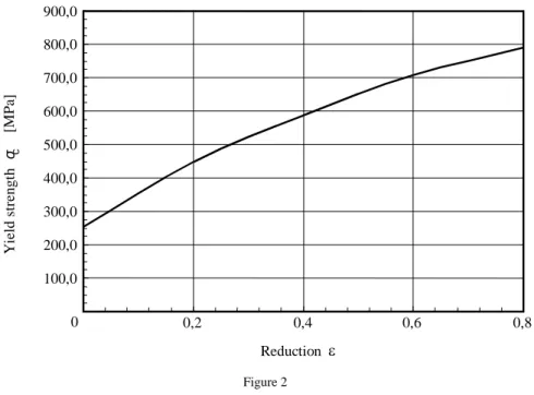
Steel hardening occurs at cold rolling. A strip hardness is describes by the compressive yield strength σc and it increases proportionally with reduction ε.

Some types of equations can describe this effect. Strip yield strength according to cubic polynomial [8] was applied in this paper:

( )

f = ³+ ² + +

= ε ε ε ε

σ_c (2)

where A, B, C, D are coefficients derived through statistical regression of data got by laboratory test on steel samples. Samples were cut from processed material between rolling stands. Initial value of yield strength (coefficient D) depends on steel chemistry and hot roll coiling temperature. The example of yield strength shape applied in the paper is shown in Fig. 2.

Figure 2 Steel yield strength shape

(Applied polynomial: σc = 313,11ε³ - 1024,5ε² + 1340,5ε + 256,65)

As was mentioned above, the mathematical model of rolling applied in the paper is based on a modified Bland-Ford model. Classical model describes the plastic deformation in roll bite (zones II and III in Fig. 3) only. Modified model considers also the elastic deformation of strip at input (zone I) and output (zone IV) of the

100,0 200,0 300,0 400,0 500,0 600,0 700,0 800,0 900,0

0 0,2 0,4 0,6 0,8

Reduction ε Yield strength σc[MPa]

roll bite, respectively (see Fig. 3). The introduced model is valid under following assumptions:

• A friction coefficient is constant within the whole roll bite,

• A contact arc between rolls and strip remains circular after roll deformation,

• The strip perpendicular sections remain straight within the whole plastic deformation zone.

A B

Elastic deformation zone (Zone I, IV)

Entry

tensile stress Exit tensile

stress

C

v hin

'_in h

hout

ψn

ψin

Neutral plane

in' ψ

σout

σin

out' h

Plastic deformation

zone (Zone II, III)

I II III IV

Figure 3

Conditions in roll bite with considering the elastic compression zone and elastic recovery zone

hin, hout strip thickness at entry and exit of the roll bite, respectively h´in, h´out strip thickness at entry and exit of roll bite plastic zone, respectively v circumferential velocity of roll

σ_in, σ_out back and front tensile stress, respectively

ψ_in angular coordinate of the strip element in the roll bite relating to the entry plane of roll bite

ψ´_in angular coordinate of the strip element in the roll bite relating to the entry plane of plastic deformation zone

ψ_n angular coordinate of the strip element in the roll bite relating to a neutral plane

Reader can find the entire derivation of modified Bland-Ford model in [5]. Only the final equations will be presented here. Specific rolling force (per unit width of strip) froll is

out e in e

roll f f f

f = + _{_} + _{_} . (3)

The specific rolling force in the plastic deformation zone f will be obtained by integration of specific roll pressure px along the whole arc of contact between strip and work rolls. Specific roll pressure at stand entry (zone II) is given by following equation

(H_in H_x)

in in in

x x input

x e

h k k h

p ⎟⎟ ^′−

⎠

⎞

⎜⎜

⎝

⎛ −

= σ^{´ μ}

´ 1 . (4)

Similarly specific roll pressure at stand exit (zone III) is determined by

1 ^x

´ μH

output x out

x x ´

out out

h σ

p k e

k h

⎛ ⎞

= ⎜ − ⎟

⎝ ⎠ ^{. (5)}

Expression Hx depends on a roll bite geometry. Its value in any place of contact arc equals

⎟⎟

⎠

⎞

⎜⎜

⎝

⎛

′

= ′

out def x out

def

x h

arctg R h

H 2 R ψ . (6)

Hin′ is obtained by substitution of value ψ_in^′ in (6).

Angle Ψ_n corresponding to the neutral plane follows from equality of px in equations (4) and (5)

⎟⎟

⎠

⎞

⎜⎜

⎝

= ⎛

def out n def

out

n R

h tg H

R

h^{´ ´}

ψ

where Hn in the neutral plane is

1

1 2 ln

1

2 ^´

´

´

´

⎥⎥

⎥⎥

⎥

⎦

⎤

⎢⎢

⎢⎢

⎢

⎣

⎡

⎟⎟

⎠

⎞

⎜⎜

⎝

⎛ −

⎟⎟

⎠

⎞

⎜⎜

⎝

⎛ −

′ −

=

in in out out

out in n in

k k h

h H H

σ σ

μ . (8)

Specific force f for plastic deformation is then given by equation

∫

∫

= ⁱⁿ

n

n

x output x def x input x

def p d R p d

R f

ψ ψ

ψ

ψ ψ

0

(9)

After substitution of (4) and (5) into (9) we get

( )

∫

∫

= ⁱⁿ

n

n

x x

in H x

out out out

x x def H x

H in in in

x x

def e d

k h

k h R d k e

h k h R f

ψ ψ

ψ μ

μ ψ σ ψ

σ

0

1

1 .

(10) The kx represents a strain resistance and is defined as

cx

kx =1,15σ , (11)

where σcx is assigned according to (2) for element of strip at position given by x coordinate. Total specific rolling force also includes forces for elastic deformation at entry fe-in (zone I) and exit fe-out (zone IV) of stand (see Fig. 3)

( )

2

_ . . .

. 4 1

in in out in

def in

in

e k

h h h R

f υE ₋σ

−

= − (12)

( )

2

_ 1 . . .

3 2

out out out def out

e R h k

f = −Eυ ₋σ . (13)

A rolling force causes deformation of processed steel and working rolls as well.

Therefore a radius of deformed working rolls has to be considered. Deformed radius according [5] is defined as

( )

( )

( )

⎜⎜

⎝

⎛

Δ + Δ + Δ +

− + −

= ₂

2 2 2

. .

. 1 . 1 16

h h

h h

h E R f

R

t out in

def π

υ ₍₁₄₎

where

(

)

out k E h

h

υ σ

− −

=

Δ 1 ². .

2

( ) (

)

t h h

h υ Eυ σ σ

. .

1− . −

=

Δ .

As could be seen in equations (9) and (14) a roll force depends on a deformed roll radius and vice versa. True values of both parameters are got by iteration. The model main issue is then actual friction coefficient. Its value is used for prediction of roll force and roll torque for next rolled coil. The critical point of iterative computation is right choice of initial conditions especially initial coefficient of friction, steel hardness and roll radius. Improper choice can cause divergence of solution and model gives no results.

With right values of friction and deformed roll radius a rolling torque could be computed. This parameter is important for checking current load of rolling motor and prediction of intended one. Knowledge of predicted load torque enables changes in rolling strategy (distribution of strip reduction and mill drives load over the tandem, respectively). There are some equations for roll torque calculation.

One of common use is as follows

⎟ ⎟

⎠

⎞

⎜ ⎜

⎝

⎛ −

+

= ∫

def out out in in x x x

def

R

h d h

p RR

M

ψ

σ σ

ψ ψ

0

2

Models used for tandem mill pre-set require fast computation methods. Values identified by the model from current rolled coil are used immediately for tandem pre-set of the next rolled coil. If the model is satisfactory quick the obtained values may be used for control of some variables on the current rolled coil.

Entire control of rolling process also includes a thermal and strip flatness models, which are not subjects of this article.

3 Application of Genetic Algorithms

Genetic algorithm falls into evolutionary algorithms group like evolutionary programming, simulated annealing, etc. [9]. It works on Darwinian principle of natural selection where biological individuals of population strife for survival and possible reproduction. Their success depends on adaptation ability. Genetic algorithm (GA) presents a stochastic optimisation method of multi parameter functions with more extremals.

GA is characterized by following properties:

• It provides wider limits of application in comparison with classical optimisation methods, because it is applicable for non-linear, discontinuous, time delay containing and similar systems. The main constraint is need of satisfactory time for off-line computation.

• It does not work with local parameters of the optimisation process but with global chromosome structure, within which parameters are coded.

• It applies searching methods that do not require information about computation control, but only definition of the objective function.

However, additional information (structure, parameter interval, initial values) may substantially decrease the time necessary for finding the optimal solution.

• Statistical transition rules are used for searching process control.

GA randomly chooses for computation the parameters falling into admissible range. The parameters combinations that suit the best to the desired solution are used in next computations. The others including divergent ones are rejected. The interval of admissible parameter combination is gradually reduced by this way.

The following approach was applied in the presented paper. Input variables for GA were

• Measured rolling force froll_act ,

• Hardening shape σ_c = f(ε) according to known grade of rolled steel (Fig. 2),

• Input thickness hin ,

• Desired thickness reduction ε ,

• Measured back and front tension value σ_in and σ_out, respectively.

A change in steel hardness and friction coefficient has the same influence on rolling force. Hence, it is not possible to identify the right value of both variables by data measured on one stand only. Therefore, the steel hardness was chosen as a fix value and friction coefficient was identified. The fitness function was defined as a minimal difference between computed roll force froll and its measured value froll_act. Exactness of the searched friction coefficient μ was increased by hybrid approach, i.e. after approximate solution by genetic algorithm a direct method such as hill climbing was applied. Further, GA enables to check the parameter combination out of searched range by mutation.

In technical praxis, the parameter values fall into known range. The fact enables to set initial intervals more precisely and increase the computational speed by this way.

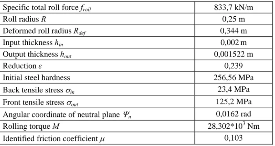
Table 1 shows an example of values applied in computation for one working point (point A in Fig. 5). The values match to the 1^st stand of five-stand tandem mill.

Table 1

Example of values applied in the computation

Specific total roll force froll 833,7 kN/m

Roll radius R 0,25 m

Deformed roll radius Rdef 0,344 m

Input thickness h_in 0,002m

Output thickness hout 0,001522 m

Reduction ε 0,239

Initial steel hardness 256,56 MPa

Back tensile stress σ_in 23,4 MPa

Front tensile stress σout 125,2 MPa Angular coordinate of neutral plane Ψn 0,0162 rad

Rolling torque M 28,302*10³ Nm

Identified friction coefficient μ 0,103

Curve of a specific rolling pressure px over the roll bite angle Ψx is shown in Fig.

4. A presence of friction hill is evident.

Figure 4

Specific rolling pressure px as a function of roll bite angle Ψx

Figure 5

Friction coefficient μ as a function of reduction ε and steel hardening q (q in p.u.) 0

0,05 0,1 0,15 0,2 0,25 0,3 0,35 0,4

0,1 0,2 0,3 0,4 0,5 reduction ε

friction coefficientμ ^{q =1.0}

0.9

1.1 1.2 1.3

A 0

100 200 300 400 500 600 700 800 900 1000

0 0,005 0,010

0,015 0,020

0,025 0,030

0,035

roll bite angle ψ [rad]

rolling pressure p [MPa]

x

x

On the real rolling mill stand the friction coefficient, steel hardness and reduction could vary in certain interval. Fig. 5 shows the parameter combinations for the same rolling force and back/front tension. The friction coefficient was calculated for steel hardening values in the range from 90% to 130% of nominal value. In Fig. 5 the steel hardening is expressed by parameter q (in p.u.) with reference value σc (according to parameters in Fig. 2).

Fig. 5 shows conditions that could be attended at next roll coil. It gives a possible pre-setting of strip reduction on the roll stand for identified friction and different steel hardness.

Conclusion

Application of genetic algorithm instead of analytical calculation offers relatively simple and fast way to determination of important rolling process parameters. In the paper, the relations amongst rolling force, tensions, steel hardening and friction coefficient at cold steel rolling has been studied. GA was used to find an actual value of friction coefficient between rolls and steel strip on the current rolled coil. The results of analysis could be used for adaptation of rolling strategy for next rolled coil. The computations were performed on PC equipped by Athlon 2,5 GHz and Genetic Algorithm Toolbox of Matlab. The time elapsed for off-line model computation for one rolling mill stand was less then 50 seconds. However, the presented approach may be applied for analysis of more rolling mill stands.

Approximately one minute of computational time could be reached with optimised algorithm for full tandem mill what is acceptable for mill presetting in real conditions.

Acknowledgment

This work was supported by the VEGA Project 1/2177/05 “Intelligent mechatronic systems”.

Nomenclature

E modulus of working rolls elasticity f function

f specific rolling force for plastic deformation (per unit width of strip) froll total specific rolling force (per unit width of strip)

fe_in, fe_out specific rolling force for elastic deformation (per unit width of strip) at entry and exit of roll bite, respectively

hx thickness of strip element in the roll gap

hin, hout strip thickness at entry and exit of the roll bite, respectively h´in, h´out strip thickness at entry and exit of roll bite plastic zone, respectively H expression given by roll bite geometry

k strain resistance

M roll torque

pavg average roll pressure p specific roll pressure

output input x

x p

p , specific roll pressure in a strip element in the roll gap at entry and exit zone, respectively

q parameter R radius of working rolls

Rdef radius of deformed working rolls v circumferential velocity of rolls ε strip thickness reduction μ coefficient of friction

σc compressive yield strength σin , σout back and front tensile stress in strip, respectively ψ angular coordinate of the strip element in the roll bite υ Poisson’s ratio

Indices

x distance along roll bite in the direction of rolling

in relating to the entry plane of the roll bite

out relating to the exit plane of the roll bite

n relating to the neutral plane

´ relating to the entry or exit planes of plastic deformation zone References

[1] D. R. Bland-H. Ford: The Calculation of Roll Force and Torque in Cold Strip Rolling with Tensions. Proc. Inst. Mech. Eng. 1948, Vol. 159, pp.

144-153

[2] W. L. Roberts: Cold Rolling of Steel. Marcel Dekker, New York and Basel, 1978, pp. 243-253

[3] A. I. Tselikov: Theory of Rolling Force Computation in Rolling Mills.

Metallurgia Moskva, 1962 (in Russian)

[4] K. Stýblo: Machinery Equipment of Rolling Mills and Drawing Mills I. ES VŠB Ostrava. 1970 (in Czech)

[5] C. C. Y. Lin, M. Atkinson: Comparison of 3 Cold Mill Rolling Force Models: The Modified Bland-Ford Model, The Roberts Model and the Stone Model. Modelling of Metal Rolling Processes. 2^nd International conference London, 1996, pp. 478-485

[6] O. Wiklund: Modelling of the Temper Rolling Process Using Finite Elements and Artificial Neural Networks. Modelling of Metal Rolling Processes. 2^nd International conference London, 1996, pp. 400-410

[7] W. L. Roberts: Computing the Coefficient of Friction in the Roll Bite from Mill Data. Blast Furnace and Steel Plant, June 1967, pp. 499-508

[8] V. Machek: Cold Roll Thin Steel Strips and Sheets. SNTL Praha 1987 (in Czech)

[9] Z. Michalowicz: Genetic Algorithms + Data Structures = Evolution Programs. Springer Verlag 1995